 ANTENNAS FROM THE GROUND UP
We have looked (and will continue to look) at antennas that present complex feedpoint impedances, that is, impedances composed of both resistive and reactive components. In the shorthand that we use for calculations, Z = R ± jX.
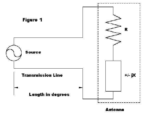
We have previously noted that a transmission line is (among other things) an impedance transformer. An impedance presented to the line as a load will appear as a different impedance at every point along the line. We can calculate precisely the value of impedance for any point along the line, as illustrated in Figure 1.
Knowing the values of impedance along a transmission is very handy. For a monoband antenna, we can select the point along a line where R is 50 Ohms and insert a compensating reactance so that we can then run coax the rest of the way to the shack. For multiband antennas fed with parallel line, we can estimate how much line to add or subtract in order to let the values fall within the range of adjustment of our ATU.
To calculate the value of impedance anywhere along a transmission line, we need only know the following: the load impedance, the characteristic impedance and velocity factor of our feedline, the line length in any units, and the frequency of operation. For ultraprecision, we can improve the result by knowing the line loss figures for the feedline type and the frequency of operation. However, for many purposes, assuming lossless lines will provide all the accuracy needed.
Now some good news and some bad news. The bad news is that, even though the necessary equation looks straightforward, the use of complex numbers (a ± jb) results in a tedious job for hand calculation. However, we have good news: we can resort either to Smith charts or to computer programs to do the heavy work for us. HAMCALC has a program called "Transmission Line Performance" that will calculate both single values and tables of values of voltage, current, and impedance (and their phases), as well as resistance and reactance along a lossless transmission line.
Actually, for impedance, we only need to look at ˝ wavelength of line, since in lossless lines, the values repeat themselves at that interval. In real lines with some loss, the values will change slightly as the line length is increased in multiples of ˝ wl.
Note, however, that values of voltage and current only change once per full wavelength. Although this fact will not affect the work we shall do in this installment, failure to appreciate it has led to some interesting errors in analyzing antennas. For example, most accounts of the ZL Special, a phased 2- element array, have viewed it as a 135° phased impedance antenna. However, antenna phasing is a product of antenna currents, not impedance. When this fact is appreciated, the antenna is more properly analyzed as a -45° phased current array.
For most low-HF wire antenna matching problems, we can focus on the impedance. The question that faces users of multiband antennas is whether the length of line in use will present to the ATU a set of values for resistance and reactance that fall within the tuning range of the ATU. The actual range of permissible values varies with the ATU network type and components. But let's arbitrarily adopt these limits: R should range from about 20-25 Ohms to several hundred Ohms while jX should run no higher than ± a few hundred Ohms. These limits would place almost all the common ATU types within their high-efficiency matching zones.
Line Length and Degrees: The first step in analyzing our situation is finding the line length we have. Actually, we need only know where along the last ˝ wl the line ends. We can calculate this length by plugging the following equations into a hand calculator:
1. Divide the total length of line by the length of ˝ wl of line, adjusted for the velocity factor (VF) of the line in use. Common 450-Ohm line has a VF of 0.95, while common 300-Ohm line has a VF of 0.80. The tables below list line lengths for various increments and frequencies. Use the figure for 180° for the nearest frequency to the one in which you are interested.
2. Throw away the integer (the part left of the decimal, if any) and save the decimal part. Multiply this number times 180 to get the number of degrees along a half wavelength of transmission line that represents the termination point of your line.
Virtually all transmission line work is done in degrees relative to a full 360° circle. 180° represents the half-circle in which we are interested. The tables below list the lengths of transmission line for various degrees along the line for selected HF frequencies that are useful for estimating your line length. Line lengths are in feet for 450-Ohm and for 300-Ohm lines.
    80-meters  3.6 MHz
L(°) L(ft): 450-Ohm 300-Ohm
 30        21.63     18.21
 60        43.26     36.43
 90        64.89     57.68
120        86.52     72.86
150       108.15     85.00
180       129.78    109.29

    40-meters  7.15 MHz
L(°) L(ft): 450-Ohm 300-Ohm
 30        10.89     9.17
 60        21.78     18.34
 90        32.67     27.51
120        43.56     36.68
150        56.27     45.85
180        65.34     55.02

    30-meters  10.125 MHz
L(°) L(ft): 450-Ohm 300-Ohm
 30        7.69      6.48
 60        5.38     12.95
 90       20.51     19.43
120       30.76     25.90
150       38.45     32.38
180       46.14     38.86

    20-meters  14.15 MHz
L(°) L(ft): 450-Ohm 300-Ohm
 30         5.50     4.63
 60       11.01      9.27
 90       16.51     13.90
120       22.01     18.54
150       27.51     23.17
180       33.02     27.80

    17-meters  18.1 MHz
L(°) L(ft): 450-Ohm 300-Ohm
 30        4.30      3.62
 60        8.60      7.25
 90       12.91     10.87
120       17.21     14.49
150       21.51     18.11
180       25.81     21.74

    15-meters  21.15 MHz
L(°) L(ft): 450-Ohm 300-Ohm
 30        3.68      3.10
 60        7.36      6.20
 90       11.04      9.30
120       14.73     12.40
150       18.41     15.50
180       22.09     18.60

    12-meters  24.95 MHz
L(°) L(ft): 450-Ohm 300-Ohm
 30        3.12      2.63
 60        6.24      5.26
 90        9.36      7.88
120       12.48     10.51
150       15.60     13.14
180       18.73     15.77

    10-meters  28.5 MHz
L(°) L(ft): 450-Ohm 300-Ohm
 30        2.73      2.30
 60        5.46      4.60
 90        8.20      6.90
120       10.93      9.20
150       13.66     11.50
180       16.39     13.80
Sample Cases: Since impedance transformations are a function of the number of degrees along a line we take a reading, regardless of frequency, we can look at some transformations that are interesting and list them in terms of degrees. You can then translate them into actual line lengths for your situation, depending on the line you are using and the frequency at which you encounter something similar to the example.
1. Mismatch with no load reactance:
Load Z = 150 ± j0 Ohms
Line Length        R ± jX
(degrees)  450-Ohms       300-Ohms
 30       193 + j223     185 + j120
 60       450 + j520     343 + j223
 90       1350 + j0      600 + j0
120       450 - j520     343 - j223
150       193 - j223     185 - j120
180       150 + j0       150 + j0
Note the symmetry of the variations of values for this line with no reactance. Still, none of the values seems to exceed what a good ATU might handle. Line length is thus not at all critical.
2. Mismatch with small inductive reactance.
Load Z = 150 + j30 Ohms
Line Length        R ± jX
(degrees)  450-Ohms       300-Ohms
 30       208 + j260     206 + j153
 60       538 + j564     419 + j226
 90       1298 - j259    577 - j115
120       380 - j475     282 - j209
150       179 - j188     166 - j90
180       150 + j30      150 + j30
Note the disruption to the symmetry due to the presence of reactance. Although the values appear reasonable, I would avoid a 90° length, if possible.
3. Mismatch with small capacitive reactance.
Load Z = 150 - j30 Ohms
Line Length        R ± jX
(degrees)  450-Ohms       300-Ohms
 30       179 + j188     166 + j90
 60       380 + j475     282 + j209
 90       1298 + j259    577 + j115
120       538 - j564     419 - j226
150       208 - j260     206 - j153
180       150 - j30      150 - j30
Notice the pattern of values and signs in the comparison of this case and the preceding one, where the only change is the type of reactance in the load.
4. Mismatch with larger inductive reactance.
Load Z = 150 + j150 Ohms
Line Length        R ± jX
(degrees)  450-Ohms       300-Ohms
 30       290 + j438     339 + j316
 60       1172 + j598    781 - j52
 90       675 - j675     300 - j300
120       213 - j321     142 - j132
150       137 - j69      115 - j8
180       150 + j150     150 + j150
This plot reveals that as the reactance goes up, part of the curve of values along the line grows quite steep. In this case, it is the first 90° of each half wavelength. The second 90° provides the best region for connection to an ATU.
5. Mismatch with larger resistance and inductive reactance.
Load Z = 600 + j150 Ohms
Line Length        R ± jX
(degrees)  450-Ohms       300-Ohms
 30       643 - j105     435 - j252
 60       435 -j180      200 - j165
 90       318 - j79      141 - j35
120       307 + j50      155 + j90
150       397 + j164     267 + j221
180       600 + j150     600 + j150
As the resistive component of the antenna feedpoint impedance goes considerably higher than the characteristic impedance of the feedline, (also making the ratio of resistance to reactance greater), the best matching region becomes the mid-region of the half wavelength line section, where the rate of change of resistance and reactance values is also the lowest. However, none of the values shown should present most ATUs with any problems.
6. Mismatch with the larger resistance and a high capacitive reactance.
Load Z = 600 - j1000 Ohms
Line Length        R ± jX
(degrees)  450-Ohms       300-Ohms
 30       138 - j371     81 - j314
 60       83 -j85        41 - j92
 90       89 + j149      40 + j66
120       89 + j149      69 + j268
150       1189 +j1216    365 + j812
180       600 - j1000    600 - j1000
As the reactance grows larger than a resistance which is already larger than the characteristic impedance of the line, the region of easiest match to an ATU shifts. For this capacitive reactance, 30° to 120° becomes the best region; for an equivalent inductive reactance, 60° to 150° would be the best region.
7. Mismatch with very large resistance and inductive reactance.
Load Z = 2000 + j2000 Ohms
Line Length        R ± jX
(degrees)  450-Ohms       300-Ohms
 30       295 - j960     116 - j606
 60       77 - j327       33 - j203
 90       51 - j51       23 - j23
120       59 + j192      28 + j143
150       138 + j587     70 + j432
180       2000 +j2000    2000 + j2000
As the resistance and inductive reactance reach the 2K level, as is common when 80-meter and 40-meter antennas are used on WARC bands, line lengths near 90° become more favorable for easy matches. Note that 300-Ohm line becomes less favorable for use, since at 90° it present a very low impedance to the ATU.
8. Mismatch with very large resistance and capacitive reactance.
Load Z = 2000 - j2000 Ohms
Line Length        R ± jX
(degrees)  450-Ohms       300-Ohms
 30       138 - j587     70 - j432
 60       59 - j193      28 - j143
 90       51 + j51       23 + j23
120       77 + j327      33 + j203
150       295 + j960     116 + j606
180       2000 - 2000    2000 - j2000
Notice the reversal of the progression of values, but not signs attached to the reactance, compared to the previous case. Also compare cases 7. and 8. to cases 2. and 3.
Cases 7. and 8. also show why the use of the 4:1 balun built into many ATUs should be avoided. With higher feedpoint impedances, the region of best match along the line encounters low impedance values. Assuming a perfect 4:1 ratio and no loss (actually, a rather poor assumption when there is significant reactance), the values seen by the ATU would be very low, either beyond the range of the ATU or subject to further losses in the network.
9. Mismatch with very large resistance and extremely large inductive reactance.
Load Z = 2000 + j10000 Ohms
Line Length        R ± jX
(degrees)  450-Ohms       300-Ohms
 30       18 - j863      8 - j556
 60       5 - j286       2 - j185
 90       4 - j19        2 - j8
120       5 + j234       2 + j162
150       13 + j707      6 + j487
180       2000 +j 10K    2000 + j10K
Note that the transformer effect of the feedlines, as their characteristic impedances become very small compared to the magnitude of the feedpoint impedance (especially the reactance), confines the high impedance values to a small region near 0 and 180°. The remainder of the line section shows very low values of resistance.
10. Mismatch with very large resistance and extremely large capacitive reactance.
Load Z = 2000 - j10000 Ohms
Line Length        R ± jX
(degrees)  450-Ohms       300-Ohms
 30       13 - j707      6 - j486
 60       5 - j234       2 - j162
 90       4 + j19        2 + j9
120       5 + j286       2 + j185
150       18 + j863      8 + j556
180       2000 - 10K     2000 - j10K
These final two cases demonstrate why half-wavelength loops and similar antennas are unusable with standard lines and ATUs. Indeed, with the end- fed Zepp, if the feedlines were not at least slightly out of balance, effecting a match with common forms of ATUs would not be possible, since the impedances presented to the feedline would be even higher.
Exploring the behavior of impedances
along a feedline can be very instructive
in estimating the most favorable line
lengths for presenting the ATU with not
only a load it can match, but one which
it can match efficiently. The samples
presented here only scratch the surface
of the subject. However, they do show
some of the emergent patterns of how
the values change with different ranges
of antenna feedpoint impedances. I
heartily recommend that you get a copy
of HAMCALC and run the values
presented with some of the antennas
we have already explored and will yet
explore in future episodes. What you
learn just might increase your antenna
system efficiency a notch or two.
Updated 11-11-98. © L. B. Cebik, W4RNL. Data may be used for personal purposes,
but may not be reproduced for publication in print or any other medium without
permission of the author.