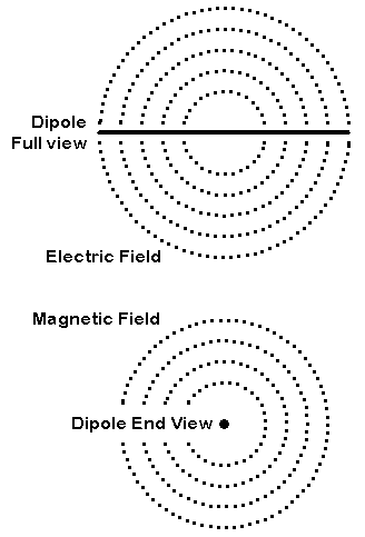
First, let's imagine a dipole. It is a typical antenna composed of a linear (straight) element. Now lets draw a circle so that the circumference touches each end of the dipole. We shall call this the E-plane. Next, let's draw a second circle and position it so that the end (either one) of the dipole makes a dot at the circle's center. We shall call this the H-plane.

Every antenna composed of linear elements has a distinct E-plane and H-plane. By convention, if the antenna has several elements, like a typical Yagi, we draw the E-plane circle so that it cuts all the elements. We center the H-plane circle on the driven element (and usually let the line of elements be horizontal across the circle).

These conventions are more than just arbitrary, because antennas composed of linear elements perform differently in each plane.

Consider an old friend, the isotropic source. The isotropic source is a hypothetical point without dimension that radiates equally well in every direction in free space--that is, space with no other objects or reflecting surfaces in it. If we were to trace a line of constant signal strength at some distance from the source, we would get equal size circles in both the E-plane and the H-plane. (In fact, we would not know just what to call the E-plane and the H-plane, except that they would have to be 90 degrees different in direction.)

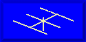
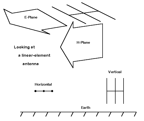
The minute we change the type of antenna, equality disappears. Let's immediately jump to the Yagi beam, since that is where we ultimately want to go. The figure below shows a hypothetical 3-element Yagi and identifies the E-plane and the H-plane. (Save the bottom of the picture for the moment.)

If we plot the performance of a typical 3-element Yagi in free space, we would want to examine both the E-plane and the H-plane. On most modeling programs, we tend to orient the antenna so that the E-plane corresponds to the azimuth and the H-plane corresponds to the elevation. Therefore, our plots will look like the figure below.

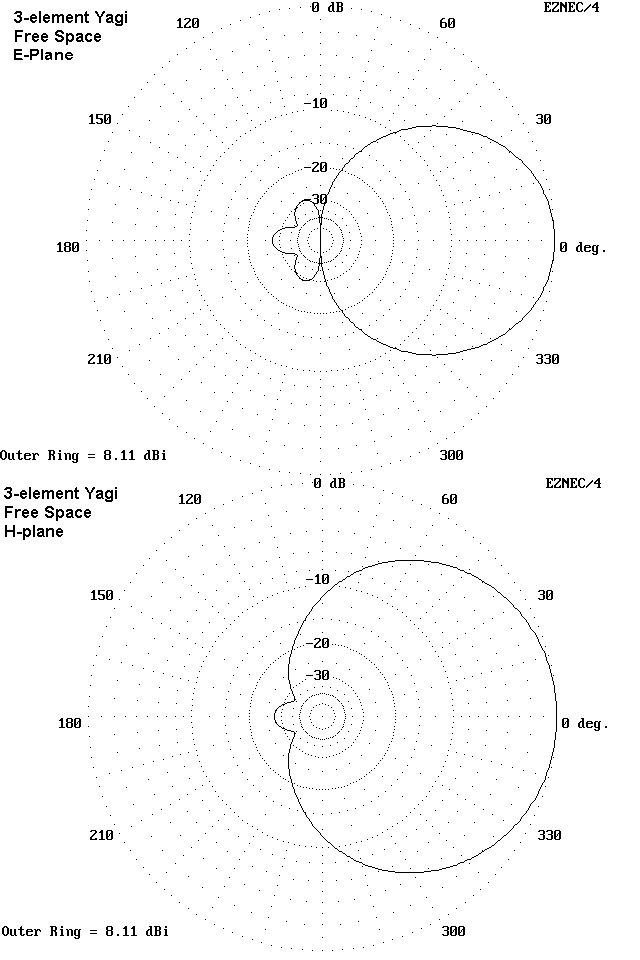
Notice that the E-plane pattern is highly confined, with a major lobe forward, some minor lobes to the rear, and strong nulls to the sides. The current magnitude and phase along the elements act together to produce this confinement of radiation.

Now examine the H-plane pattern. Since there are no linear element ends (and resultant current magnitude and phase level pattern along the element) to confine the radiation, the pattern is nearly a circle, simply displaced forward of the driven element. The variation of the pattern from a true circle is a product of the interaction of the radiation from the three elements.

These patterns will be replicated with some variation for every antenna composed of linear elements in a plane. A very long UHF Yagi or a complex phased array of Extended-Double-Zepp elements might narrow the beam width in the E-plane from the 3-element Yagi's 50-60 degrees down to less than 20 degrees. Large arrays with many elements often show somewhat ragged edges to the equal-signal strength lines. But allowing for these variations, the E-plane and H-plane free space patterns of the antennas will show their kinship.

Now return to the original picture and examine the bottom. Here we have introduced the earth and have placed our Yagi over it in two different orientations. On the left, the plane of the antenna (the E-plane) is parallel to the earth and we call the orientation horizontal. On the right, the plane of the antenna is at right angles to the earth and we call the orientation vertical.

What is crucial about the difference is that when the antenna is horizontal, it is the H-plane which the earth cuts off in the form of reflecting signals that would have been directed downward. The E-plane radiation pattern is largely unaffected. When the antenna is vertical, the E-plane is cut off in the form of signal reflection, and the H-plane pattern is unaffected.

We can show the consequences of each with a small sample. Let us place the Yagi 1 wavelength above the earth, as measured by the position of the boom that holds the elements in alignment. If the antenna is horizontal with respect to the earth, then the antenna pattern looks like that in the following figure (assuming, as we do in all modeling, a flat, uncluttered earth surface).

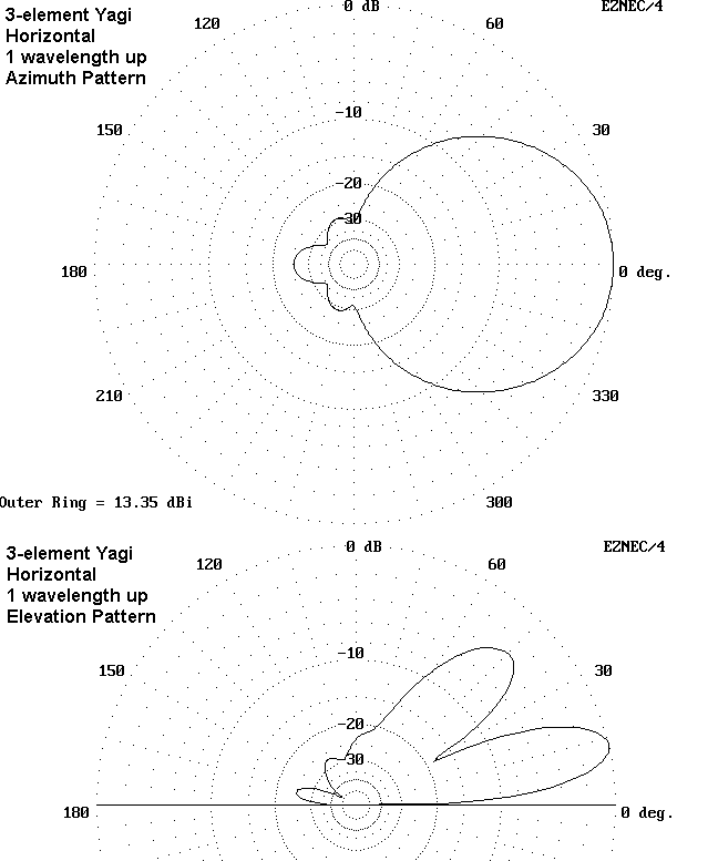
The patterns above are the azimuth and elevation patterns of the Yagi oriented horizontally with respect to the earth's surface. First of all, note that the azimuth pattern shape is almost the same as the E-plane pattern in free space. The beam width of 50-60 degrees coincides closely to the free space value.

The only significant difference is the gain, which is now something over 5 dB higher than in free space. Arrayed over good, but not perfect ground, the gain is typical for 3-element Yagis 1 wl up. The quality of ground makes a small and operationally insignificant difference in the antenna's gain. Larger variations show up as the antenna height is changed between, say, 0.5 wl and 2 wl. Gain maxima occur roughly at 5/8, 1 1/8, and 1 5/8 wl heights, while minima occur at 7/8 and 1 3/8 wl heights. These maxima and minima become indistinct the higher we raise the antenna.

Where the added signal strength comes from is revealed by the elevation pattern. The signal which in free space would have radiated downward is reflected by the earth (with only a very small loss for horizontally oriented antennas). It combines with the direct signal radiated upward. At some points, the two signals combine in phase and add to create a lobe. At other points, the signals combine out of phase to create a null.

The lobes and nulls form a regular pattern. The general formula for lobes and nulls is

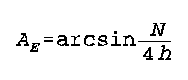
where Ae is the elevation angle of the lobe or null, N is an integer indicating the number of the lobe or null from lowest upward, and h is the antenna height in wavelengths or a fraction thereof. Odd integers indicate lobes and even integers indicate nulls.

For convenience, the following table provides the elevation angles of the first lobe, usually the strongest, and second lobe for horizontal antennas at heights of 0.5 wl up to 2 wl.

Antenna height      Angle of first      Angle of second
 in wl                   lobe                lobe
     0.5                 30 deg              none
     0.75                19                  90 deg
     1.0                 14                  49
     1.25                12                  37
     1.5                 10                  30
     1.75                 8                  25
     2.0                  7                  22

The table gives elevation angles in whole numbers for two reasons. First, a fraction of a degree makes no operational difference in a lobe that has considerable vertical dimension, as shown in the elevation pattern above. Second, the real properties of the antenna and of the ground will alter the exact angle of maximum radiation, especially at lower heights. For example, NEC-4 models of 3-element Yagis over average earth tend to show maximum elevation angles of radiation between 24 and 26 degrees, rather than the calculated 30 degrees. These difference tend to wash out as the antenna is raised higher. However, this chart will serve as a general guide to expectations. (Note: Hasan Shiers, N0AN, has posted similar information on one of the antenna-related lists.)

Now let us consider what happens if we build the Yagi in a vertical orientation with the boom 1 wl up. The resultant patterns are these:

As the azimuth pattern demonstrates, the side-to-side pattern resembles very closely the H-plane pattern of the free space model. The beam is about 100 degrees wide between -3 dB power points, about twice as wide as the beamwidth of the Yagi when horizontally oriented. However, compare the maximum gains of the horizontal and vertical Yagis: the vertical Yagi has for this particular case almost 5 dB less gain.

Because the element ends are within 3/4 wl of the ground, the gain deficit relative to the horizontal Yagi of identical design is fairly high. As the height of the antenna increases, the gain deficit diminishes for antennas many wavelengths up as would be the case with most VHF/UHF Yagis. A 2-meter 3-element Yagi 5 wavelengths up shows a gain differential of about 1.5 dB between vertical and horizontal orientations. Moreover, because vertically oriented linear antennas are more dependent on ground quality than horizontal antennas, the degree of gain deficit will vary with the ground quality. Again, the degree of differential will diminish as the antenna height is increased.

The elevation pattern of the vertically oriented Yagi also differs considerably from that of the horizontal Yagi. For low Yagis with boom heights under 2 wl, the first two lobes tend to blend into a front. The angle of maximum radiation is 10 degrees for the case of the Yagi with a boom 1 wl up, but that point is part of a broad, flatted field face of considerable vertical dimension. The vertical beamwidth of the elevation pattern is about 30 degrees.

These properties do not make the vertically oriented HF Yagi useless by any means. Granted, for rotatable beams atop high towers, horizontal orientation has become an accepted standard for good reason. However, not every amateur installation can raise such Yagis. Wire antennas in fixed positions are often necessary for a variety of reasons. An array of 4 vertically oriented Yagis would provide world-wide coverage. With some ingenuity, one might use a single driven element with only 4 other vertical wires. By using inductive and/or capacitive reactance, the other 4 wires can be converted into directors or reflectors--or detuned to not be part of the array. Hence, world-wide coverage might be achieved with a 4-way switch, a few relays, some transmission-line stubs, and one or more weather proof boxes to house the junctions. Even with tubular elements, the cost will be considerably less than a tower and rotator, and the maintenance ease is likely to be considerably greater.

Such systems have been built in the past and will be built again. Their exact design goes far beyond the point of this note, which has been to provide some basic acquaintance with the consequences on far field patterns of orienting a Yagi horizontally and vertically. If the patterns displayed here add a bit to your rational expectations of antennas, they will have done their work.

Supplementary Note:
The Evolution of the E-Plane and the H-Plane

The names for the plane derive from basic antenna fields, electrical and magnetic. For a succinct mathematical treatment of these fields, see "Fundamentals of Antennas," by Henry Jasik in Johnson (ed.), Antenna Engineering Handbook, 3rd Ed, pp. 2-1 to 2-7. For a more thorough non-mathematical treatment, see The ARRL Antenna Book, pp. 2-7 to 2-9.

Linear antenna elements produce two types of fields: the E or electrical field, in which lines of force roughly parallel a linear element, and the M or magnetic field, in which lines of force are tangential to the linear element. The figure above is suggestive of the fields, but--like all the other 2-D approximations I have encountered--is not wholly accurate. Note that the lines in the figure are rounded and I just said they are parallel. Neither is strictly true.

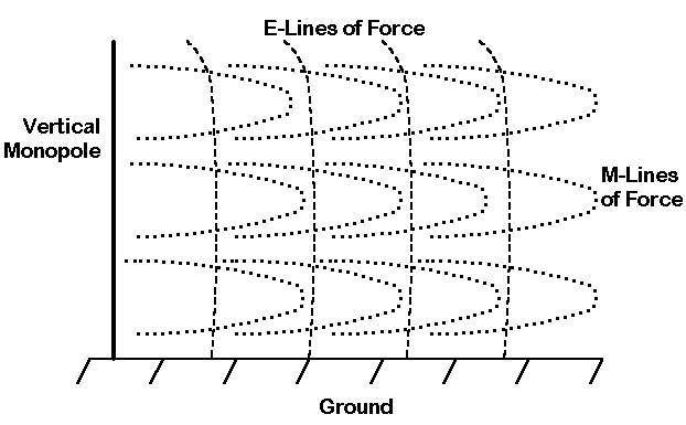
This next figure gives a different slant on the fields from the perspective of a vertical monopole and adapted from the ARRL figure 23-1. I have modified the figure to give a sense of lines of force. Electrical lines, running top to bottom are nearly straight, while magnetic lines circle the antenna element.

Now place a dipole is free space and think about the electrical and magnetic fields. The lines of force of one project roughly in line with the antenna element and this is the E-field. The lines of force of the other project in circles about the element at right angles to it, and this is the M-field.

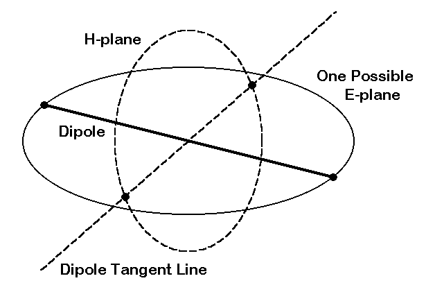
The circles in the figure above show one way of looking at the fields. One major line of force of the magnetic field will intersect a tangent line drawn through the center of the dipole. I have added big dots to associate the circle with the correct line.

The lines of force for the electric field are in the plane of the antenna, which means that for illustrative purposes, they touch the ends of the antenna. This defines part of the E-field.

The E-field defines and creates the E-plane. The M-field defines and creates the M-plane.

Now for the crooked shift: when we consider very distant field strength--the far field--we consider virtually only the E-field. However, we preserve the E-plane and the M-plane that the different fields have created and lent their names to.

The above far field pattern is taken in an E-plane of a dipole in free space. It records on a line of equal field strength a pattern of interest to use. This particular pattern is an E-plane pattern labeled in dB.

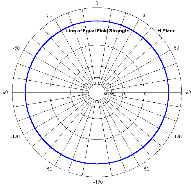
Since we are in free space, we can also take a 360-degree H-plane pattern, that is, a pattern at right angles or tangential to the linear dipole. However, this field records the electrical field (not the magnetic field), just as did the E-plane field.

The circularity of the H-plane pattern tells us that we could have taken any slice through the element and create another E-plane at some angle to the one we chose to use.

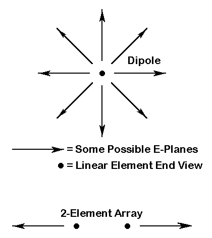
The figure above indicates that there are an indefinitely large number of possible E-planes and E-plane patterns with a single dipole element, which the figure shows end-on. In free space, one is as good as another.

However, the instant we go to 2 elements, the elements reduce the E-plane to one field in the plane of both elements. As shown in the figure, the E-plane cuts both elements equally. From this point, you can move back to the representation in the very first figure in the note on polarization. The arrow heads on the plane representations are simple indicators that the antenna in question has directional gain and a rear null. The actual E-plane and H-plane extend indefinitely far in their 2-dimensional extensions.

All of this is bound to raise some questions. For example, suppose three elements are not in line, but make some kind of triangle when viewed end-on. Suppose an antenna element has wires that go every which-a-way.

Since we are dealing with conventions, we might as well add another. Complex antenna geometries are usually initially referenced to their intended application over the ground. Then a line parallel to the ground can be drawn through the array of elements viewed end-on. This is the E-plane. If such a line cannot be drawn because of the orientation of the elements, then a parallel to high current node of the antenna can be drawn and this becomes the E-plane. A second plane at right angles to the first can be drawn to cut at least some of the elements and this becomes the conventionalized H-plane.

Some antennas, like the delta loop fed as a vertically polarized 1-wl array, defy even this treatment. However, by the time we get to this advanced state of affairs, we have added the ground to our system and can reference the antennas to it. In such cases, we speak of the less confusing vertical and horizontal polarization of radiation from the antenna. Talk of E-plane and H-plane is best suited to simple antennas in free space. They are reminders of certain fundamental concepts in antenna operation. However, for many complex arrays of elements, it is far less confusing to view them over a ground and then, if necessary, export the vertical and horizontal notions back into free space, referencing them to the X, Y, and Z coordinates of a familiar cartesian system.

Updated 4-22-98, 10-13-98. © L. B. Cebik, W4RNL. Data may be used for personal purposes, but may not be reproduced for publication in print or any other medium without permission of the author.

Go to Amateur Radio Page