 Modeling the Dual Rhomboid
Interest in the design has periodically peaked in various parts of the overall communications field, including amateur VHF and UHF efforts and the TV reception (cable and individual) industry. For either application arena, improved rhombics offer the potential for an inexpensive antenna (some wire and wood) with high gain and relatively easy construction.
Cliff Buttschardt, K7RR, graciously provided me with some background material appearing in the October, 1976 CATJ, and other information has appeared in 73 and QST. The article's references include several Radio-Electronics articles between 1953 and 1960, mostly referenced to TV uses of the rhombic. As well, there are references to Laport's original papers in the RCA Review (March, 1952, and March, 1960). Bill Parker, W8DMR, wrote on the "Dual Rhombic for VHF-UHF" in 73 for August, 1977, and the information there was edited and relayed by Emil Pocock, W3EP, in his VHF column (p. 89) in QST for March, 1997. The reason for the resurgence of interest in 1997 stems from the 1296 MHz version of the dual rhomboid built by Dayton Johnson, W0OZI, which won the 1996 Central State VHF Conference antenna gain test with a measure 17.3 dBi gain value. (See QST for December, 1996, p. 90.)
Although Laport developed several advanced multi-element rhomboid antenna designs (hand-calculated), the most favored for its ease of implementation is the dual rhomboid. (The elements are rhomboids, but not true rhombi, since the sides are not necessarily perfectly parallel.) It is on the dual rhomboid that I shall concentrate, since it presents a number of challenges to the antenna modeler.
In this note, I shall focus on the 1296 MHz version of the antenna derived from the work of W8DMR as revised by W3EP, since that is likely the antenna design most accessible to most hams. Apparently, W3EP scaled the antenna design from a 1255 MHz ATV version in Parker's article. Among the claims made for the antenna are the following of interest to an inveterate modeler. 1. The gain may be 20 dB better than a dipole. 2. The antenna allows for "sloppy" construction without jeopardy to success.
In all of this background material, no mention is made of the antenna's front-to-back ratio. Moreover, Laport's theoretical calculations and HF applications of the antenna suggested that terminating resistors for each section of this traveling wave design should be about 660 Ohms and yield a net feedpoint impedance of about 330 Ohms. In ham writings, this has been uncritically translated into 600 Ohm resistors and a 300-Ohm feedpoint impedance.

To see how this works, see Fig. 1, a general outline--with dimensions--of the 1296 MHz version appearing in QST. The two rhomboids are offset from each other--left and right--by a small distance at their terminating points so that the separate patterns maximize the main forward lobe and minimize troubling side lobes that are characteristic of single rhombic designs. Both rhomboids are fed in parallel. Laport's original designs called for no separation between the "upper" and the "lower" wires, but only insulation at the crossing points. Typical ham practice has mounted the two rhomboids on opposite sides of a frame, usually about 3/4" to 1" thick (at UHF, a minimum size for sturdiness).
At 1296 MHz, a wavelength is about 9.11" long, so the length of the antenna from feedpoint to terminating resistors is about 8.4 wl and the maximum width is about 4.7 wl. (This may account for the fact that no ham has yet constructed a rotating HF version of the antenna.) At 1296 MHz, the antenna is about 77" long and 42.5" wide--quite manageable dimensions.
There are two sets of antennas to be explored: the QST model and the CATJ versions derived directly from Laport's analysis. In this part, I shall look only at the QST model. One important reason for this is that modeling the antenna is tempting for anyone with a basic modeling program using NEC-2. However, creating a useful (I shall not use the term "precise") model of the Laport dual rhomboid is not so easy a task as it may seem, and I shall point to some dangers in the enterprise before seeing what the QST model yields.
Modeling a rhomboid shape with a feedpoint and two terminating resistors also requires small distortions of the ideal acutely angled points to the geometry. For the 1296 MHz model, I used 1" multi-segment wires at the points in which to place the resistors and the source. Although an inch seems small compared to a total length of 77", it is 11% of a wavelength and thus cannot be neglected as a potential error source. These wires used at least 3 segments (and some as high as 7) to ensure centering of the source and resistors and to ensure that segments adjacent to the source and load were the same length of the source and load segments.
The wires for the longer and shorter sides are equally highly segmented. I developed two models, the chief difference between them appearing in Fig. 1A.

Model A brings the two wires on each side of the feedpoint to a common junction. This is a somewhat dangerous modeling practice, since the wire segments closest to the junction intersect--even for small diameter wire--along an appreciable portion of the segment. This can create modeling errors. Convergence to a reasonable, but not perfect, degree required models using nearly 1600 segments.
Model B changes all of the angles to right angles, minimizing the mutual wire penetration effect. It may also reflect ham construction using a wood frame. These models converged reasonable with about 800 segments.
However, the results obtained from just the change in feedpoint area treatment differ by enough to warrant presentation of both sets of figures. For many purposes, the differences may not make a difference, but that is not something that a modeling exercise can establish from the outset. For example, the feedpoint impedance of Model A is higher than the theoretical 300 Ohms by about as much as the feedpoint impedance of model B is below that value.
In all azimuth patterns, to add to the slowness of model runs, I used a 0.1 degree resolution. The patterns of rhombics of any form are too complex for the 1-degree resolution we habitually use with Yagis.
Interestingly, in no case did I obtain anything close to the 20 to 27 dB gain over a dipole. All modeling was done in free space using copper wire losses, so a comparison with a free space dipole should reduce the reported figures by about 2.1 dB. This does not make the dual rhomboid a poor antenna, since 16 dBi free space gain from a hank of wire and a few slats of wood is still excellent performance potential.
For reference, here is the description of Model B as used below.
Dual Rhombic-QST 3-97, p89                Frequency = 1296  MHz.

Wire Loss: Copper -- Resistivity = 1.74E-08 ohm-m, Rel. Perm. = 1

              --------------- WIRES ---------------

Wire Conn.--- End 1 (x,y,z : in)  Conn.--- End 2 (x,y,z : in)  Dia(in) Segs

1   W8E2  -0.500,  0.000,  0.000  W2E1  -0.500,  0.000,  0.500    # 12    2
2   W1E2  -0.500,  0.000,  0.500  W3E1 -15.250, 27.500,  0.500    # 12   75
3   W2E2 -15.250, 27.500,  0.500  W4E1   5.500, 77.000,  0.500    # 12  120
4   W3E2   5.500, 77.000,  0.500  W5E1   6.500, 77.000,  0.500    # 12    3
5   W4E2   6.500, 77.000,  0.500  W6E1  21.250, 50.000,  0.500    # 12   75
6   W5E2  21.250, 50.000,  0.500  W7E1   0.500,  0.000,  0.500    # 12  120
7   W6E2   0.500,  0.000,  0.500  W8E1   0.500,  0.000,  0.000    # 12    2
8  W15E2   0.500,  0.000,  0.000  W9E1  -0.500,  0.000,  0.000    # 12    3
9   W1E1  -0.500,  0.000,  0.000 W10E1  -0.500,  0.000, -0.500    # 12    2
10  W9E2  -0.500,  0.000, -0.500 W11E1 -21.250, 50.000, -0.500    # 12  120
11 W10E2 -21.250, 50.000, -0.500 W12E1  -6.500, 77.000, -0.500    # 12   75
12 W11E2  -6.500, 77.000, -0.500 W13E1  -5.500, 77.000, -0.500    # 12    3
13 W12E2  -5.500, 77.000, -0.500 W14E1  15.250, 27.500, -0.500    # 12  120
14 W13E2  15.250, 27.500, -0.500 W15E1   0.500,  0.000, -0.500    # 12   75
15 W14E2   0.500,  0.000, -0.500  W7E2   0.500,  0.000,  0.000    # 12    2

              -------------- SOURCES --------------

Source    Wire      Wire #/Pct From End 1    Ampl.(V, A)  Phase(Deg.)  Type
          Seg.     Actual      (Specified)
1           2     8 / 50.00   (  8 / 50.00)      1.000       0.000       I

              --------------- LOADS ---------------

Load      Wire      Wire #/Pct From End 1      R (Ohms)       X(Ohms)
          Seg.     Actual      (Specified)
1           2     4 / 50.00   (  4 / 50.00)     600.000         0.000
2           2    12 / 50.00   ( 12 / 50.00)     600.000         0.000

Ground type is Free Space
One question of interest is whether wire size plays any significant role in antenna performance. The easiest way to find out is to run identical antenna dimensions with various wire sizes. Here are the results for 1296 MHz, using the prescribed 600-Ohm terminating resistors. In the tables that follow, gain is the free space value in dBi, F-B is the 180-degree front-to-back ratio in dB, B/W is the -3 dB beamwidth in degrees, F/S is the ratio of the forward lobe to the most major side lobe in dB, and the Feed Z is the source impedance.
Model A  (1581 segments)

AWG       Gain      F-B       B/W       F/S       Feed Z
Size      dBi       dB        deg       dB        R+/-jX
12        16.23     15.99     10.0      10.24     347 - 81
14        16.25     16.55     10.0      10.23     372 - 58
16        16.29     16.90     10.2      10.26     391 - 46
18        16.22     17.49     10.2      10.23     411 - 33
20        16.17     18.18     10.2      10.21     429 - 23
Although the gain does not change in practical terms, it does show a peak with #16 copper wire. Interestingly, the QST article suggested that #12 would be the smallest wire likely to be used. I am not certain that is a sound statement, since the #16 version of the model also showed the highest front-to-side lobe ratio. Note also the increasing front-to-back ratio and feedpoint impedance as the wire size decreases. These phenomena are likely effects of increasing wire losses, which do not affect gain significantly.
Model B  (797 segments)

AWG       Gain      F-B       B/W       F/S       Feed Z
Size      dBi       dB        deg       dB        R+/-jX
10        15.71     14.98     10.3      10.74     186 - 17
12        15.76     15.54     10.4      10.66     200 -  8
14        15.80     16.20     10.4      10.57     213 -  1
16        15.81     16.92     10.4      10.48     226 + 10
18        15.81     17.71     10.4      10.40     239 + 18
20        15.80     18.59     10.4      10.33     251 + 26
The antenna gain for this model is systematically about a half dB lower than for Model A, and the reported source impedance is below 300 Ohms. Interestingly, the front-to-back ratio is almost identical for each wire size between the two models. One of the reasons that I tend to trust Model B more than Model A is the smaller excursion of reactance with the changes in wire size (noting that I added #10 wire to Model B just to see what would occur). Moreover, the gain peak is less pronounced and the front-to-side ratio makes a steady progression downward as the front-to-back ratio climbs.

Fig. 2 provides a free space azimuth pattern for Model A, which is virtually identical to the pattern for Model B with a slight adjustment of gain. Despite the careful calculations made by Laport, this version of his work cannot suppress the main side lobe by more than 10 dB relative to the main lobe.

It is interesting to compare the azimuth plot to a free space vertical (or elevation) plot for the antenna (Fig. 3). In this plane, we see a broadening of the main forward and rear lobes (to about 30 degrees between -3 dB points). We may also note that the largest side lobe also appears in this pattern, giving the impression that it may form a cone around the main lobe.
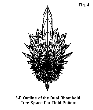
A 3-D view of the pattern, shown in Fig. 4, can give us a better view of what is happening with the main side lobe--or side lobes. First, we must allow for the fact that the reduced resolution of the 3-D pattern converts smooth petals into crystalline points. Nonetheless, we can see that the main side lobe is actually a series of undulating lobes and nulls around the main lobe. (Those given to such things can make any sort of desired Rorschach test out of the 3-D pattern.)
To some degree, then, the dual rhomboid is sensitive to wire size in the 1296 MHz model we are examining. We may increase the front-to-back ratio by decreasing the wire size. We should also wonder what effect we might achieve by changing the values of the terminating resistors. The next data set for both models explores two versions of each model: #12 wire and #16 wire--that latter because it coincides with the gain peaks shown by the preceding data. One of the basic questions to pose is whether there is a value of terminating resistor that will maximize the front-to-back ratio. The following data set systematically reduces the terminating resistor values in 100-Ohm increments from 600 to 200 Ohms.
Model A  (#12 wire; 1581 segments)

Res.      Gain      F-B       B/W       F/S       Feed Z
Size      dBi       dB        deg       dB        R+/-jX
600       16.23     15.99     10.0      10.24     347 - 81
500       16.21     17.77     10.0      10.17     338 - 81
400       16.17     20.23     10.0      10.07     327 - 83
300       16.14     21.97     10.0       9.95     313 - 85
200       16.09     18.31     10.0       9.77     295 - 89

Model A  (#16 wire; 1581 segments)

Res.      Gain      F-B       B/W       F/S       Feed Z
Size      dBi       dB        deg       dB        R+/-jX
600       16.29     16.90     10.2      10.26     391 - 42
500       16.26     19.15     10.2      10.17     379 - 46
400       16.23     21.91     10.2      10.06     364 - 51
300       16.20     21.50     10.2       9.92     346 - 58
200       16.17     16.37     10.2       9.74     323 - 68
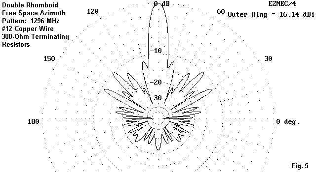
Despite differences occasioned by the smaller wire size occasioning more rapid property changes than the larger wire size, the two tables show an interesting coincidence. The maximum front-to-back ratio occurs with a load between 300 and 400 Ohms--closer to 300 Ohms for the #12 wire and closer to 400 Ohms for the #16 version. Fig. 5 shows the resultant azimuth pattern for the #12 version with terminating resistors of 300 Ohms.
Model B  (#12 wire; 797 segments)

Res.      Gain      F-B       B/W       F/S       Feed Z
Size      dBi       dB        deg       dB        R+/-jX
600       15.76     15.54     10.4      10.66     200 -  8
500       15.74     17.64     10.4      10.55     194 -  8
400       15.72     20.92     10.4      10.42     186 -  8
300       15.69     24.15     10.4      10.23     177 -  9
200       15.67     18.91     10.4      10.00     165 - 10

Model B  (#16 wire; 797 segments)

Res.      Gain      F-B       B/W       F/S       Feed Z
Size      dBi       dB        deg       dB        R+/-jX
600       15.81     16.92     10.4      10.48     226 + 10
500       15.79     19.64     10.4      10.37     218 +  9
400       15.77     23.64     10.4      10.23     209 +  8
300       15.75     23.11     10.4      10.06     197 +  7
200       15.74     16.59     10.4       9.83     182 +  5
As with Model A, Model B shows its maximum front-to-back ratio with terminating resistors between 300 and 400 Ohms. The consistency between the source impedance values for the two wire sizes gives me additional reason to trust Model B more than Model A, even though the primary trends coincide.
Whether the source impedances reported by Model B are accurate to a real antenna involves a number of variables. Some of those variables include limitations of the model itself, as described earlier. Other variable emerge from the construction process itself. Ideally, the support structure for the antenna should be RF-transparent at 1296 MHz. Likewise, construction practices should involve no metal supports--not even nails--close to the wire. Even a few 1-inch brads can add up to a wavelength of nails very quickly. As a consequence, any real version of the dual rhomboid is likely to show a source impedance somewhat at variance of even the most precise model.
One final question that occurred to me resulted from the claims that the dual rhomboid forgives sloppy construction. In more precise form, one may ask to what degree the antenna may be frequency sensitive. As a partial answer to this question, I ran Model A through a few wire sizes but on the ATV frequency of 1255 MHz, about 3% lower. (Some claims for the broad-banded nature of the antenna suggested that +/- 40% of the design frequency would be usable.) The following table compares the results for Model A at 1296 and 1255 MHz for 3 wire sizes, using the standard 600-Ohm terminating resistors.
Model A  (1581 segments)

Freq.     AWG       Gain      F-B       B/W       F/S       Feed Z
MHz       Size      dBi       dB        deg       dB        R+/-jX
1296      12        16.23     15.99     10.0      10.24     347 - 81
1255      12        16.20     19.37     10.6      10.30     313 -108

1296      16        16.29     16.90     10.2      10.26     391 - 46
1255      16        16.26     21.48     10.8      10.20     362 - 80

1296      20        16.17     18.18     10.2      10.21     429 - 23
1255      20        16.14     23.96     10.8      10.12     409 - 61
With respect to gain, no especially frequency sensitivity can be found. However, the front-to-back ratio with a given value of terminating resistor is quite frequency sensitive. At the lower frequency, the 600-Ohm terminating resistors are close to optimal for maximizing the front-to-back ratio. Moreover, the added capacitive reactance at the source is quite evident for all of the wire sizes.
Whatever the final evaluation of the adequacy of these models, it is clear that the Laport dual rhomboid antenna is not quite the "set-and-forget" item that some sources portray it to be. Its properties vary with wire size, terminating resistor value, and frequency. Whether any of those variations are significant to a given operation can only be judged by reference to the operating specifications.
Moreover, the realizable gain from at least the QST version of the antenna is considerably less than claims derived from theory (which rarely takes into account wire losses). What I hope to squeeze time for is a look at the dimensions derived more directly from Laport's work--perhaps something in the 100 MHz range (about 8 times longer than the 1296 MHz model). When I am semi-satisfied with models of that antenna, I shall add Part 2 to this report on modeling the dual rhomboid.
Updated 8-14-99. © L. B. Cebik, W4RNL. Data may be used for personal purposes, but may not be reproduced for publication in print or any other medium without permission of the author.