
A considerable while ago, I did a modeling investigation into "The Effects of Antenna Height on Other Antenna Properties: A Computer Study," Communications Quarterly, 2 (Fall, 1992), 57-79. However, I still find that folks are not wholly familiar with the change of elevation lobes as one changes the height of a horizontal antenna. So I thought a note might be in order.
By now, most folks are familiar with how to derive the angle at which lobes and nulls exist for any given height. The angle for any lobe of a horizontally-oriented antenna can be estimated from the simple equation
where ALN is the angle of the lobe or null above the horizon and h is the antenna height in wavelengths or fractions thereof. Odd values of N represent lobes (points of maximum radiation) while even values of N represent nulls (points of minimum radiation). Hence, if N=3, the lobe in question is the second above the horizon.
The existence of lobes and the angle at which each shows maximum gain is, of course, valuable information. With this data, we can choose (if we have a choice) the most optimal height for an antenna for a desired angle of radiation relative to a favored propagation path at the frequency of interest.
What is less well known is the fact that changing the height of the antenna has other consequences as a result of the changing pattern of lobes that develop between some given minimum height and some given maximum height. Between a height of 0.5 wl and a height of 1.5 wl, the maximum gain of a dipole may shift by over 0.5 dB. For a beam antenna, the front-to-back ratio can swing by as much as 10 dB. For antennas more complex than dipoles, design will have much to do with the change in properties with changes in height, but even within a single design class--for example, Yagis with the same number of elements--there are variables.
Since the point of this note is to illustrate the phenomenon, I can give the best advice up front: for any given antenna, it is best to model it at a series of heights to understand the potential variations of performance. In some cases, the results may make a difference in the selected installation height; in other cases, the results may give the installer a free hand.
     7.0 MHz                  14.0 MHz                 28.0 MHz
Gain  Source Impedance   Gain  Source Impedance   Gain  Source Impedance
dBi   R +/- jX Ohms      dBi   R +/- jX Ohms      dBi   R +/- jX Ohms
2.12  72.1 - j 0.5       2.12  72.2 - j 0.4       2.11  72.3 - j 0.3
When we place this antenna over average ground (Cond. 0.005 S/m; D.C. 13), and change its height in 1/8 wl increments from 0.5 wl to 1.5 wl, we get the following table of values.
             7.0 MHz                14.0 MHz               28.0 MHz
Height    Gain Source Imp.       Gain Source Imp.       Gain  Source Imp.
WL        dBi  R +/- jX Ohms     dBi  R +/- jX Ohms     dBi   R +/- jX Ohms
0.5       7.57 66.8 - j10.5      7.33 68.0 - j 9.8      7.21  68.8 - j 9.6
0.625     8.00 63.7 + j 3.5      7.82 64.3 + j 2.8      7.74  64.6 + j 2.3
0.75      7.39 75.3 + j 6.7      7.31 74.7 + j 6.3      7.28  74.4 + j 6.3
0.875     7.26 78.3 - j 3.1      7.18 78.1 - j 2.5      7.13  78.1 - j 2.0
1.0       7.80 69.9 - j 6.0      7.68 70.5 - j 5.6      7.61  71.0 - j 5.4
1.125     8.05 67.1 + j 1.4      7.94 67.5 + j 1.1      7.89  67.8 + j 0.8
1.25      7.70 73.8 + j 4.0      7.64 73.5 + j 3.8      7.62  73.4 + j 3.8
1.375     7.56 76.2 - j 2.0      7.50 76.0 - j 1.6      7.47  76.1 - j 1.2
1.5       7.88 70.8 - j 4.3      7.80 71.2 - j 3.9      7.75  71.5 - j 3.8
For easier reading, the following graph tracks the gain curves for the three frequencies. (See Fig. 1.) The curves are "spiky" because of the interval between readouts. Smaller increments would have produced smoother curves, but no essential difference in the data.

Although incidental to the present exercise, the reduction in gain with frequency increase for exactly scaled dipoles is a useful reminder that material and ground losses do not frequency-scale as perfectly as antenna dimensions for resonance. The increased losses with frequency show up not only in the gain curves, but as well when one compares the maximum and minimum reactance excursions at the three frequencies: A lesser excursion indicates a higher loss. Although the differences are not operationally significant in this case, the general trend is worth remembering.
More significant to our exercise is the gain differential of the dipole at 0.875 wl and at 1.125 wl: nearly 0.8 dB at 7 MHz. The curve shows gain peaks at 0.625 and 1.125 wl antenna height, with minima at 0.875 and 1.275 wl. The differential between maxima and minima decreases with antenna height increases, although the curve is distinct well beyond a height of 2 wl.
Where the power goes when the gain of the lowest lobe decreases is illustrated in Fig. 2.
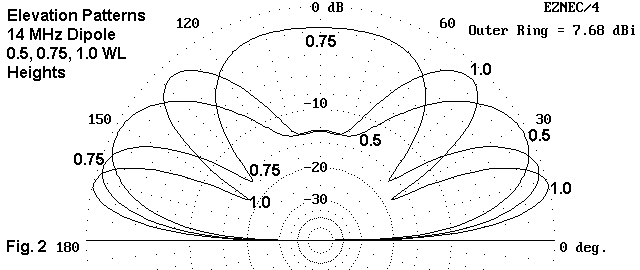
The elevation pattern for the dipole at a height of 0.5 wl shows a single "fat" lobe in each direction. At a height of 0.75 wl, the second lobe has emerged. However, it is a large lobe of energy pointed almost straight up, more suitable for NVIS use than for DX skip. The vertical dimension of the lower lobes has decreased. If we assume that the area under each curve is the same (which is not precise, but reasonably close), and that total power is represented by this area, then the amount of energy sent straight up with the mergence of the new lobe can be seen to be considerable.
When the antenna reaches a height of 1 wl, the second lobe has moved downward, while the lowest lobe has moved slightly outward, while still showing a reduction in its vertical dimension. Maximum gain is the highest of the three situations. However, note the slight center (90-degree elevation) bulge in the pattern. A new lobe will emerge in the nearly vertical plane to reach a peak, with a reduction in gain in the lowest lobe, at about 1.375 wl. The cycle of lobe emergence continues indefinitely with further increases in antenna height, but each succeeding new elevation lobe has a decreasing effect on the gain of the lowest lobe.
With a simple dipole, there is a rough reverse correlation between gain maxima and minima and the source impedance maxima and minima. That is, the source impedance is highest when the gain is lowest--and vice versa--as we move up the scale of increasing antenna heights. Like the gain highs and lows, the impedance highs and lows grow less extreme with increases in height.
Let's begin with a standard 2-element driver-reflector Yagi. The one we shall examine uses a 0.230 wl driver and a 0.254 wl reflector, spaced 0.125 wl apart, with 1.81E-3 wl element diameters. The material is aluminum. We shall test the antenna over average ground only at 14 MHz, after resonating the antenna in a free space model. In tabular form, our results look like this:
Height         Gain      F-B Ratio      Source Impedance
WL             dBi       dB             R +/- jX Ohms
Free Space      6.06     11.05          36.2 - j 0.9
0.5            10.74     12.39          40.3 - j 3.3
0.625          11.14      9.62          34.2 - j 4.0
0.75           11.15      9.98          33.7 + j 0.5
0.875          11.24     11.88          38.1 + j 1.4
1.0            11.47     12.11          38.3 - j 1.7
1.125          11.59     10.38          35.3 - j 2.7
1.25           11.55     10.30          34.6 - j 0.2
1.375          11.57     11.53          36.7 + j 0.6
1.5            11.68     11.79          37.6 - j 1.3
Graphically, the pattern of gain and of the front-to-back ratio appear as shown in Fig. 3.
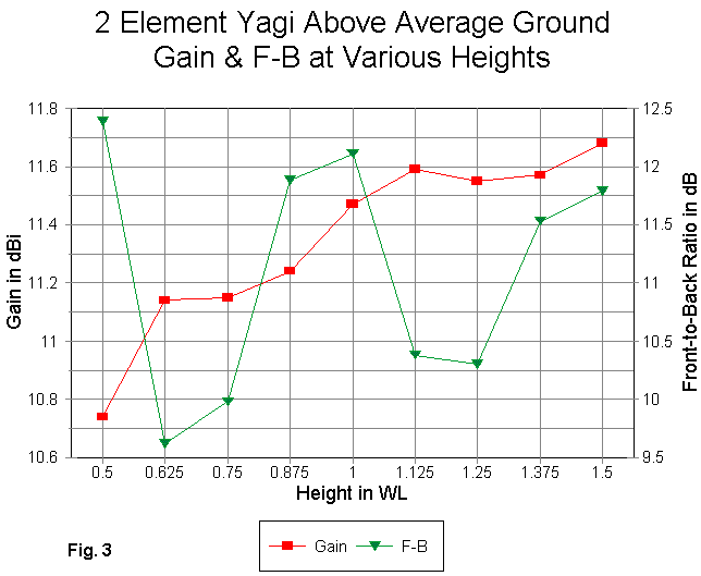
The gain maxima continue to occur at the 0.625 and 1.125 wl marks, but the gain minima for this antenna are less distinct and somewhat offset from the dipole model. Minima occur almost 1/8 wl below those for the simple dipole--a function of the Yagi's second element. Since different designs for even 2-element Yagis will place the two elements at different spacings, we cannot assume that Fig. 3 represents all possible designs. If the height vs. antenna parameter relationship is of interest, it should be checked for each specific design.
The front-to-back pattern of maxima and minima are especially variable among designs. If you examine the table, you will discover a rough correlation between the maxima and minima for both the front-to-back ratio and the source impedance.
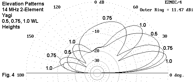
The developmental pattern for new lobes follows that of the dipole, with adjustments for the directional nature of the 2-element Yagi. As shown in Fig. 4, the new lobe in the 0.75 wl height pattern provides power largely in a vertical direction. At a height of 1 wl, the new lobe bends forward, with a consequential flattening of the lower lobe.
Height         Gain      F-B Ratio      Source Impedance
WL             dBi       dB             R +/- jX Ohms
Free Space      8.11     27.31          25.7 - j 0.9
0.5            12.29     25.35          24.6 - j 0.7
0.625          12.85     24.58          25.8 + j 0.2
0.75           13.08     36.69          26.6 - j 1.0
0.875          13.23     30.15          25.6 - j 1.6
1.0            13.39     25.19          25.1 - j 0.9
1.125          13.50     25.63          25.6 - j 0.3
1.25           13.56     32.37          26.2 - j 0.9
1.375          13.62     29.32          25.7 - j 1.3
1.5            13.67     25.46          25.3 - j 1.0
We can show the gain and front-to-back curves graphically in Fig. 5.
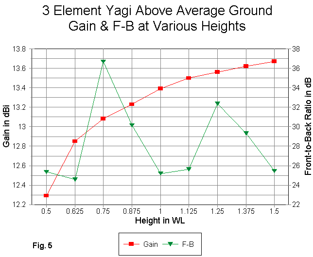
For this well-designed 3-element Yagi, the gain curve shows no gain dips. However, by carefully tracing the curve, one can see very slight reductions in the rate of gain increase in the 0.75-0.875 wl region and again in the 1.25-1.375 wl region. These values are of no operating significant whatsoever for this design, but are only remnants that establish the origins of the Yagi in the basic dipole.
The front-to-back curve is another matter. It tends to peak where the gain minima would have been--at the 0.75 wl and the 1.25 wl region. For this design, the front-to-back peaks tend to correspond to source impedance peaks. However, the overall excursions of both the resistive and reactive components of the source impedance are very small.
Let us contrast this design with another 3-element Yagi design that has been pressed for gain. Consequently, the front-to-back ratio is lower than our first design, and the source impedance is very low. The director is 0.236 wl long, the driver is 0.241 wl long, and the reflector is 0.251 wl long, with 0.253 wl director-driver spacing and 0.152 driver-reflector spacing. The elements are 2.41e-3 wl diameter and are aluminum. The operating parameters of this antenna at 14 MHz over average ground are as follows:
Height         Gain      F-B Ratio      Source Impedance
WL             dBi       dB             R +/- jX Ohms
Free Space      8.30     11.26           5.6 + j 6.2
0.5            12.28     13.70           5.9 + j 6.4
0.625          12.88     12.66           5.8 + j 6.0
0.75           13.12     10.82           5.5 + j 6.1
0.875          13.31     11.05           5.5 + j 6.4
1.0            13.51     12.15           5.8 + j 6.3
1.125          13.64     12.06           5.7 + j 6.1
1.25           13.69     10.97           5.5 + j 6.2
1.375          13.75     10.99           5.6 + j 6.3
1.5            13.83     11.72           5.7 + j 6.3
We can show the gain and front-to-back curves graphically in Fig. 6.
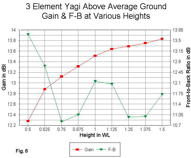
Like the first 3-element Yagi design, this alternative shows a steady rise in gain with antenna height, with only a slightly greater flattening of the curve in the regions of lower gain in a dipole. However, the pattern of front-to-back ratio is almost precisely the reverse that of the first 3- element Yagi: the new model shows maxima and minima just where the first model shows the opposite. If there is a lesson here, it is that each design must be checked for its own characteristics. However, there is a rough correlation between front-to-back maxima and minima and corresponding highs and lows in the source impedance values.
The second Yagi design cautions us to presume nothing about the performance of an antenna design. This lesson is especially important in the development of interlaced Yagis for multi-band operation. The complex interaction of the elements--and the assembly with the ground--can yield some surprises--not to mention the emergence of advantageous heights and heights to avoid.
Let's look at a 2-element quad with a driver having director sides 0.126 wl long and reflector sides 0.133 wl long, spaced 0.125 wl. The elements are copper and are 1.93E-4 wl diameter. As with the other antennas, we shall run the model over average ground at 14 MHz.
Height         Gain      F-B Ratio      Source Impedance
WL             dBi       dB             R +/- jX Ohms
Free Space      7.32     21.58          94.4 + j 0.4
0.5            11.36     18.75          99.4 + j 4.1
0.625          11.99     21.12          97.4 - j 4.0
0.75           12.15     27.06          91.0 - j 1.8
0.875          12.29     21.70          92.3 + j 3.2
1.0            12.53     19.99          96.8 + j 2.5
1.125          12.71     22.15          96.2 - j 1.8
1.25           12.71     24.30          92.5 - j 1.1
1.375          12.74     21.46          93.0 + j 2.2
1.5            12.85     20.40          96.0 + j 1.9
We can show the gain and front-to-back curves graphically in Fig. 7.
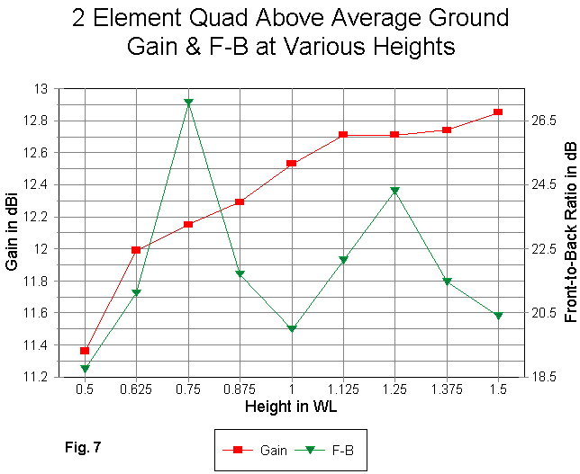
More like the 2-element Yagi, the quad shows deviations from a smooth curve in the regions where the dipole shows reductions in gain. However, the front-to-back curve resembles that of the optimized 3-element Yagi in the placement of maxima and minima. What both these models share in common is having been optimized for a best combination of gain and front-to-back ratio.
Nonetheless, the quad has a feature unlike the other models: the front-to- back ratio maxima correspond to source impedance minima and vice versa. (The other models examined had a direct correlation between source impedance and front-to-back ratio.) Hence, we once more encounter patterns that dictate the checking of each new antenna design, if the performance at various heights is of interest.
In our little foray into the variables of antenna performance with changing antenna height, we have looked only at the formation of the second lobe in the 0.75 to 0.875 wl region. For reference, it may be useful to look at both the quad and the optimized 3-element Yagi at 1.25 wl, where the third lobe begins to emerge. See Fig. 8.
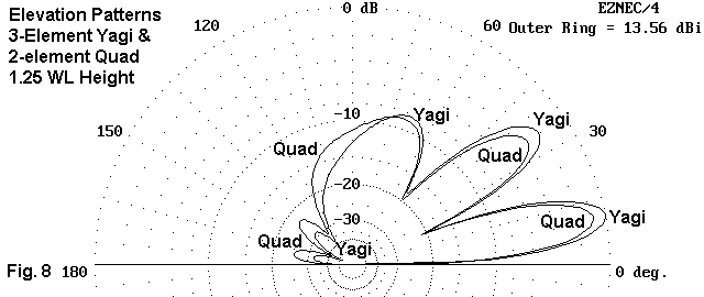
The higher gain and directivity of the 3-element Yagi has some consequences of note relative to the quad. At a height of 1.25 wl, the Yagi top lobe is already bent forward, while the quad top lobe shows more area in the vertical direction. Otherwise--with allowance for the gain and front-to- back differential, the lobes show an exact correspondence. Once more, let us uses the area within the overall pattern as a rough and inexact gauge of total power. If the Yagi has more gain, it comes from expending less in the upward direction than from the differences in the rear lobes. (Note that relative beam widths for the two models has not been taken into account in this comparison.)
Some horizontal antenna designs are immune (or almost immune) to the effects of lobe development in the vertical plane. Most of these designs involve phased elements. The in-phase fed elements of the 8JK flat-top tend to yield a cancellation of vertical radiation. Hence, the gain curve is smooth as antenna height is increased. Even the Lazy-H and the extended Lazy-H, vertically arranged in-phase fed 2-element arrays show a great reduction in vertical radiation compared to dipoles and parasitic arrays. Notable but lesser reductions in vertical radiation occur with some arrays phased at other angles.
Although almost any horizontal antenna can be related to dipole performance with respect to lobe emergence, specific antenna designs will add enough variables to the mix to require separate height analysis for each one. In most cases, the region from 0.75 wl to 0.875 wl should be avoided, if possible. But even this generalization is subject to modification based on the analysis of a specific design.
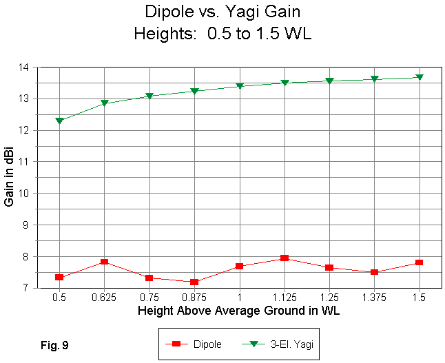
Fig. 9 compares the gain at heights of 0.5 to 1.5 wl above average ground. We notice the smoothness the of the Yagi curve and the slight wave in the dipole curve. The question is this: can we make use of this data? Of course we can. A graph of the gain differentials shows us how in Fig. 10.
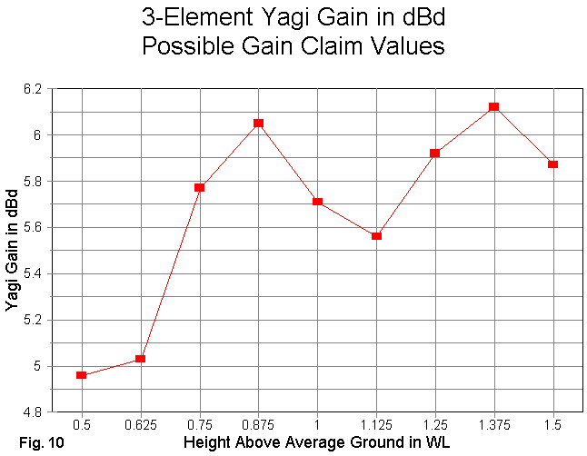
By carefully selecting the 1.375 wl height, we can claim that the antenna has a gain of over 6.1 dBd. Note that only at that height and at 0.875 wl does the Yagi achieve its free space gain advantage of 6 dB or more. (All gain figures are taken at the elevation angle of maximum radiation or "take-off" angle.)
With equal care, a competitor might choose to claim that other antenna designs, including this one, have a gain of only a little over 5 dBd, using (at the extreme) the 0.626 wl height as the evidence. A more conservative competitor might claim that "other" 3-element Yagis of the same boom length have only a little over 5.5 dBd gain, using the 1.125 wl height data. Now, this competitor might also claim 6.1 dBd gain for his product, using the 1.375 wl height data. Of course, heights of data backing the claim would not appear in advertising literature.
Which would you buy: a 3-element Yagi with just over 5.5 dBd or one with 6.1 dBd? Of course, the competitor's design is identical to the original.
This exercise is not designed to comment on the practices of any manufacturer. Instead, it is designed to graphically illustrate that the use of gain values in dBd must be handled with exceptional care and with complete data for the conditions of establishing the numbers. Only then can the reader be in a position to evaluate competing claims. This point is not just applicable to advertised antennas. It applies with equal force to reports of antenna designs that appear in journals of all levels, from magazines for beginners to peer-reviewed engineering journals. The point is equally applicable to antenna comparisons made at different times: the results may not be directly comparable unless all of the testing conditions--including antenna height--are the same for each testing session.
Gain in dBd must always have a warning label: HWC. Handle with care.
Updated 4-30-99, 5-7-99. © L. B. Cebik, W4RNL. Data may be used for personal purposes, but may not be reproduced for publication in print or any other medium without permission of the author.