 Part IV: Series Circuits and Reactance
Arithmetically, we have two ways of handling reactance as part of the load. For some purposes, it is better to treat the two components together as a complex number typically shown as R +/- jX, where both R and X are given in ohms. In other applications, we can separate the two. When it comes to ATUs, reactance can usually be treated separately at the load end of the design.
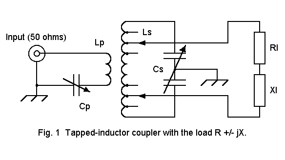
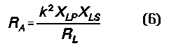
Figure 1 shows once more out basic link-coupled tuner circuit. We have opted initially to use a simplified tapped inductor scheme for matching lower resistive loads to the full tuned circuit. As a first step, let's consider once more a 1500 ohms resistive load connected in parallel with the resonant parallel L-C circuit. At 7 MHz, with a secondary inductor of 12 micro-H (with a reactance of 528 ohms at that frequency) and a primary inductor of 1.2 micro-H (53 ohms reactance), the resonant capacitance in the secondary was 43 pF. We chose our 1500 ohms resistive load (RL) to go with an assumed k of 0.6 for a mutual reactance (XM) of 100 ohms. The secondary loaded Q was 2.8 or so to obtain about 54 ohms for RA.
However, Figure 1 shows a complex load impedance with the series values RL +/- jXL. normally, complex antenna feedpoint impedances and impedances to be found along the length of a given feedline are specified in series terms. In order to evaluate the situation, we need to convert the complex load into parallel equivalents, using the standard conversion equations:


Note that XP is in parallel with XLS and XCS, the reactances of the secondary coil and capacitor, respectively. If the equivalent parallel load reactance, XP, is inductive, then the total inductive reactance is the parallel combination of XLS and XP. Likewise, if the equivalent parallel load reactance is capacitive, then the total capacitive reactance is the parallel combination of XCS and XP.
Since calculators have a convenient inverse (1/X) key, it is normally much more convenient to convert parallel reactances to parallel susceptances, which simply add, in order to obtain the value of the parallel combination. In other words,

The following table illustrates what happens to the parallel combinations for our standard 1500-ohms resistive load when there are various series reactive loads, XL, of moderate proportions.
 Parallel Inductive and Capacitive Reactances with Load Reactances
RL=RS         XL=XS         RP            XP            XLT           XCT
1500          -500          1667          - 5000        528           -477
1500          -200          1527          -11450        528           -505
1500           200          1527           11450        505           -528
1500           500          1667            5000        477           -528

Note:  all values in ohms.

Table 1.  Total parallel inductive (XLT) and capacitive (XCT) reactances with load
reactances.
With modest (XL < 1/3 RL) reactive components to the load, the parallel equivalent resistive load across the tuned circuit does not change very much. The values of reactance that now compose the tuned circuit are sufficiently different to require adjustment of the variable capacitor to restore resonance. Where the reactive load is capacitive, the capacitor must show less capacitance and more capacitive reactance to make up for the loss occasioned by the parallel equivalent capacitive load reactance.
Where the reactive load is inductive, the capacitor must show more capacitance and less reactance to resonate with the reduced inductive reactance occasioned by the parallel equivalent inductive load reactance. However, these values are not the optimum to effect a transformation to 50 ohms in the primary. Hence, other adjustments of the tuner components may be needed to effect a good match, including moving to a different tap of the coil.
When the load is transformed from a lower value to a higher value needed by the secondary tuned circuit to effect a transformation to a desired primary impedance, not only is the resistive component increased in value, but so too is the reactive component. For most cases, the chief effect of this transformation is to reduce the effects of the secondary variable capacitor in compensating for the changes in total parallel reactance. This effect is especially pronounced with inductively reactive loads which, when treated in parallel equivalent form, move the inductive reactance of the tuned circuit components well off their optimum values. The capacitor setting required may result in a considerable offset, resulting in a resonant frequency (in terms of XLS = XCS) significantly removed from the operating frequency. The result will often be higher circulating currents within the tuned secondary circuit and lower efficiency of power transfer to the load. However, these losses are ordinarily very small if a high Q coil is used and the loaded Q of the circuit is held low.
The conditions of maximum efficiency cannot always be achieved, especially if the ratio of reactance to resistance in the load becomes great. Moreover, the higher the Q of the secondary circuit, the smaller the frequency range over which a single set of adjustments are usable. These conditions hold true whether one is using a tapped inductor or a capacitor divider as the means of effecting a match with a wide range of load values.

In 3A and 3B, we treat the reactance at the terminals in its series form. If the reactance is inductive, we insert a mechanically linked pair of capacitors--one in each side of the line--to provide an equal but opposite value of capacitive reactance. If the reactance at the terminals is capacitive, we insert a pair of series inductors in the line to provide equal but opposite reactance. The net reactance is zero, and the tuner sees a resistive load.
Series compensation is normally mechanically difficult, especially with the use of variable components. First, each side of the line must be broken to insert the proper compensating component. Dual components are necessary to preserve line balance. Second, mechanically linked components are bulky--inductors even more so than capacitors. Series compensation is rarely used.
In 3C and 3D, we treat the reactance in its parallel equivalent form. This conversion permits us to place either a coil or a capacitor across the line to provide an equal but opposite reactance value to cancel the parallel equivalent reactance presented by the load. Very usually, single ended components are employed in this function. Because of slight imbalances in the structure of such components, the line balance may be slightly disturbed, but ordinarily not enough to hinder circuit or transmission line operation. The switching or tapping methods should remove both sides of the compensating component when it is not in use.
The use of advance reactance compensation is necessarily reserved for very high load reactances that challenge the ability of the variable capacitor in the secondary circuit to effect a match or which unduly raise the Q of line or the coupler circuit. Series reactances in this range normally convert to parallel-equivalent low to moderate reactance values which are within the range of reactance compensation by good quality everyday components. When series reactances are themselves low to moderate, most coupler designs can easily accommodate them. In addition, their parallel equivalent values may be beyond the range of compensating components.
For example, in Table 1, a series reactance of 200 ohms, is easily handled by the coupler design used in our running example. However, compensation by parallel components is another matter. If the load reactance is capacitive, it would require a compensating inductance of 260 micro-H, and if the load reactance is inductive, it would require a compensating capacitor of 2 pF at the 7 MHz operating frequency. Needless to say, neither of these are practical values to find in variable components.
Every feedline is also an impedance transformer all along every 180-degrees of its length. If the antenna feedpoint impedance exactly matches the characteristic impedance (ZO) of the feedline, then the impedance along the line is constant at the value of line ZO. If the antenna feedpoint impedance differs from the ZO of the line, then the value of impedance, in terms of R +/- jX, varies all along each 180-degree length of line. This is true, whether the antenna feedpoint impedance is purely resistive or a combination of resistance and reactance.
With a complex feedpoint impedance that does not match the ZO of the feedline, there may be some line lengths that present easy combinations of R +/- jX for a given coupler design to handle and other lengths that present values that may exceed the coupler design limits. Hence, selecting something close to an optimum line length may enhance the ability of the tuner to compensate for the reactance and maximize power transfer to the feedline.
Let's use a challenging antenna case to see how this works. A certain antenna presents a feedpoint impedance at 7 MHz of 1828 + j1826 ohms. Assuming that we are using 450-ohms parallel feedline with a velocity factor of 0.95, we can obtain the following table of impedance values along a 180-degree length of line. (Similar tables at 5-degree intervals can be obtained from a program included with the VE3ERP HAMCALC collection. The values assume lossless line, but for planning use with antenna tuners, the accuracy will be more than adequate.)
                     Resistance and Reactance Along a 450-ohms Feedline

                     Line Length                 Impedance
              Degrees       Feet          Resistance (ohms)    Reactance (ohms)
                0            0              1828                 1826
               10            3.7            3173                -1291
               20            7.4             857                -1513
               30           11.1             334                - 970
               40           14.8             179                - 662
               50           18.5             116                - 469
               60           22.3              85                - 333
               70           26.0              69                - 226
               80           29.7              60                - 136
               90           33.4              55                -  55
              100           37.1              55                   22
              110           40.8              57                  101
              120           44.5              64                  187
              130           48.2              77                  285
              140           51.9             100                  407
              150           55.6             146                  571
              160           59.3             249                  820
              170           63.0             545                 1245
              180           66.7            1828                 1826

Table 2.  Resistance and reactance along a 450-ohms feedline for a typical antenna.
If the line length must be more than 1/2 wavelength, just add increments of 66.7' to the lengths listed to get just about the same values. But now that we have the table, what do we look for?
We are seeking a length of line where the reactance values are low. Achieving a zero level of reactance is unnecessary, but values under 200 ohms would be well within the range of virtually any coupler. Notice that the reactance passes through zero in two places. However, reactance curves are not orderly sine waves. Between 0 and 10 degrees, the reactance rapidly changes from a high inductive value to a high capacitive value. Since this makes finding the right length difficult, we shall avoid this transition. Between 90 and 100 degrees, the reactance passes slowly through 0. Hence, the exact line length becomes far less critical. In feet at 7 MHz, the ideal length is close to 36 feet long, but plus or minus 7-10 feet either way would not challenge the coupler.
Since almost any multi-band antenna can be modeled with reliable ballpark accuracy on all intended bands of use, it is possible to develop a full set of feedline charts plotting the excursions of resistance and reactance. Simply plug the modeled feedpoint impedance for each band into the impedance transformation program and print out a chart. By examining the reactance progressions for each band, it may be possible to find a minimal number of line lengths that will permit an easy match for the coupler.
Under very fortunate circumstances, you may find a single line length that will physically work with the antenna in question and also provide reasonable reactance levels for the tuner. If two or more lengths are requires, then switching or manually adding in the required line lengths for the band or bands which need them becomes the next order of business. Of course, all of the rules for treating parallel line carefully apply to this system. Hence, the actual switching system becomes a challenge for the creativity of the individual station operator. Line switching is often very much cheaper and less complex than installing and switching pre-coupler compensating inductors and capacitors.
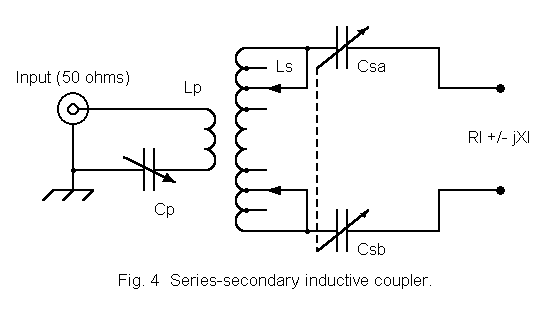
Typical inductor and capacitor values are so similar to those for parallel tuners that we can retain our chosen values in the running example: 12 micro-H for the secondary and 1.2 micro-H for the primary. Their respective reactances are 528 and 53 ohms. The series reactance of the capacitor will likewise be 528 ohms at ideal resonance, and hence, each section must be able to provide half this value, just as in the parallel tuner. For a total capacitance of 43 pF, each section must be able to reach 86 pF. However, the capacitor cannot be a simple split stator-common rotor model, but must be a pair of independent units mechanically driven as a unit. Some apparent split stator models are actually of this design and use a jumper for achieving a common rotor, which is then grounded for balance across the line. With the series connection, the capacitor sections must each float (that is, be well insulated from a common ground).
From one perspective, the equations that drive a series circuit look quite different from those that drive the parallel circuits we have been examining. Yet, as an exercise in "what goes around comes around," let's look at these equations.
For a series tuned inductively coupled tuner, where the secondary is presumed to be resonant, the input or primary impedance is a function of the reactance of the mutual inductance and the load resistance:

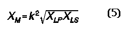
Once more, XM is related to the coefficient of coupling (k) in this way:
Unlike a parallel tuned circuit, the loaded or working Q of a series-tuned circuit is


Series-tuned couplers are normally used with low coefficients of coupling to effect matches of low impedances to the coupler input impedance. If we let the desired value of RA be the same as the value of the primary inductor reactance (about 50 ohms),
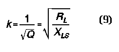
Using equation (9) with our running example circuit values, we can develop a small table of reasonable values of k to effect a 50-ohms match with various load resistances.
                     Values of k for a 50-ohms Match with Various Loads

                     Load Resistance      Loaded Q      Required k
                          (RL)            (XLS/RL)      for 50-ohms match
                          100                5.3          0.44
                           50               10.6          0.31
                           25               21.1          0.22
                           10               52.8          0.14

Table 3.  Values of k for a 50-ohms match with various loads where XLS = 528 ohms.
The table clearly shows the progression of values, but also shows a rapidly increasing Q as the load resistance to be matched goes down. High Q has the same effect with series- tuned circuits as with parallel-tuned circuits: the required settings become very narrow and must be changed with small excursions of the operating frequency.
Additionally, the presence of reactance in the load has the effect of requiring the tuning capacitor to be reset to restore resonance. Where the load reactance is capacitive, the overall component reactance at resonance can be maintained, because shifting the capacitor to a higher capacitance setting reduces its reactance to compensated for the line reactance: the net capacitive reactance is the same as the inductor's reactance at resonance. However, if the load reactance is inductive, it adds to the reactance of the secondary coil. This situation requires a change in the capacitor setting to a smaller value to match the combined inductive reactance to restore resonance. The effective reactance at resonance is higher, thus increasing the circuit Q and increasing the inconveniences (and possible problems) associated with high Q.
The most convenient way in most typical amateur circumstances to rid the load of its high reactance with a series tuned coupler is to alter the line length. However, in doing so, we can usually find a line length with a higher load resistance as well as a lower load reactance. Since parallel tuned coupler designs are available for loads of 50 ohms or even slightly less, the end result has been a gradual decline in the use of series-tuned coupler circuits.
In the end, the parallel-tuned link coupler, with either a tapped secondary or a capacitor- divider for handling a wide range of load impedances, is the circuit of choice for inductive couplers. The tapped secondary version, while useful for manual operation in multi-band units, is often used with single-band couplers, say, for 160 meters. Once the right settings are found, no further manual changes in taps are normally needed during operation. Such tuners are also cheaper to build, since soldering taps to coil turns is normally less expensive and easier to accomplish than finding a suitable differential capacitor for the alternative load network.
For multi-band couplers, the capacitor divider provides continuous front panel adjustment for changes of load impedance. With a multi-section ceramic wafer switch to set the inductor size for each band, along with the tuned circuit variable capacitor and the optional series input capacitor, this design can be reset from band to band quickly as one changes operating frequencies.
We have now looked into the basic theory and fundamental circuitry of inductively coupled
ATUs. The remaining questions we need to examine concern component values and ratings,
construction practices, and measurements to assure best results. Perhaps we can do all this
in just one more session.
Updated 11-28-97. © L. B. Cebik, W4RNL. Data may be used for
personal purposes, but may not be reproduced for publication in print or
any other medium without permission of the author.