 Part I: Inductive Coupling
Just as interest grows, the number of available link-coupled tuners continues to dwindle. Moreover, parts for such tuners grow scarcer. Along with the depletion in tuners and parts, there is also a scarcity in available information on the operating and construction principles underlying the link-coupled tuner. This series of articles is designed at least to correct the information part of the problem. Restoration of the parts supply and the inventory of complete units is another problem entirely.
Some hams have attempted to avoid balun losses by placing a 1:1 balun at the source side of the tuner and floating the unit to provide a nearly balanced output to the load. Common- mode currents continue to be a problem in many installations.
Rarely have hams attempted to build balanced networks for their tuners. Balanced Ls, Tees, and PIs are certainly feasible, but at a cost. In some schemes, component values double; in others, mechanical linkages present construction complexities. Such units remain rare.
For many hams, the tuner of choice for parallel transmission line systems is the inductively-coupled tuner. It yieldss efficient power transfer to a naturally balanced output. Moreover, it provides a degree of isolation from the line due to the inductive or magnetic coupling. This latter feature often suffices to attenuate out-of-band RF from strong local sources.
However, not just any old tank and link will make a satisfactory tuner. We have largely forgotten the fundamental principles behind good tuners of this type. Perhaps the high point of available information was in the 1960s. In my own collection of old ARRL Antenna Books, the 9th Edition of 1960 contains an account that is both mathematically and practically superior to the account of my next older edition, the 7th of 1955. By the 13th edition of 1974, much of the material had been digested to make room for the single ended network and baluns and has remained essentially unchanged since that time. The link coupled transmatch still in the 18th edition of the ARRL Antenna Book of 1997 is the same as that in my 1982 ARRL Handbook (although few have noticed that the front panel photo has changed appearance over the years, while the top view shows the original unit).
These notes on the evolutionary ups and downs in available link tuner information are not at all a criticism of ARRL publications. Quite to the contrary, other handbooks in English present considerably less information on these tuners and their principles. Yet the information is available from a combination of sources. The 1960 ARRL Antenna Book account is, of course, crucial. One source especially useful on inductive coupling is George Grammer's A Course in Radio Fundamentals which ARRL published as a full text in 1972. The source behind this treatment--as it is for so many other matters relating to radio fundamentals--is Terman's Radio Engineers' Handbook. They all make good reading for those interested in going beyond the treatment presented here.
So perhaps it is time to go back to the beginning and reintroduce the link coupler from the ground up. Nothing in these notes will be new, but only a restatement of principles and practices gleaned from the sources. At most, I shall be adding some tables and examples to the account in order to give the applicable equations some real meaning. The tables may also allow those who do their math intuitively a chance to see the trends of values to permit more accurate ballpark extrapolations. Moreover, I shall not try to give a fully integrated mathematical account, but simply present certain of the most useful equations that either explain tuner operation or permit calculations useful to constructing such tuners. Since most will be practical simplifications, there will be gaps in mathematical progressions of derivation. But then, our aim is to provide--so far as possible--a practical grounding in inductive tuner principles.
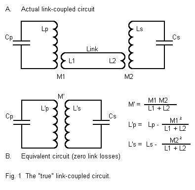
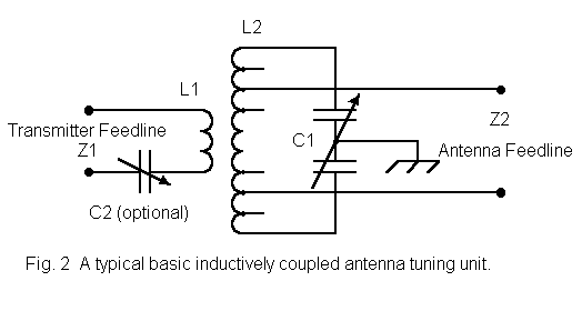
In isolation, the antenna tuning unit (ATU) shown in Figure 2, is an inductively coupled impedance matching network. Even though networks dominate the output circuits of modern transmitters, the concept of coefficient of coupling may still be applied to the inductively coupled circuit, and to that degree it is still correct to call these ATUs link-coupled tuners.
However, the old name often carries with it an attitude: the small coil is merely the link and as such is not of great importance. Calling the unit an inductively coupled impedance matching network gives equal importance to both the primary and secondary inductors. That is crucial for understanding this class of ATUs.
We shall keep the old name, since that is only a war of words, but we shall lose the old attitude. That way, the link coupler and the inductively coupled impedance matching network will become one and the same. Now if we only knew what is going on with inductive coupling, we would be in good shape to understand the link coupler.
Two key concepts arise in this connection. The first is mutual inductance (M), that is, the voltage induced in the second coil by the rate of current change in the first. M is measured in Henrys, just as is the inductance of the coils. Often neglected is the fact that mutual inductance can be measured. First measure the inductance of the two coils individually and well apart from each other. Second, fix the positions of the coils with respect to each other, connect the coils in series, and measure the total inductance. Finally, reverse the series connections and remeasure the inductance. Note that inductance-measuring devices ordinarily use an internal alternating current signal source to make their measurements.
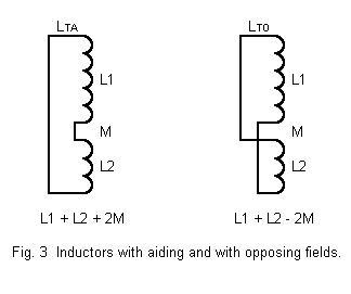
If the two coils as positioned have any mutual inductance, as illustrated in Figure 3, then the two readings will differ, one being larger than the sum of the inductances of the coils as measured independently, the second smaller than that sum. The larger reading (LTA) records the coils connected so that the fields are said to aid each other; the smaller (LTO) records the connections that oppose each other. In fact, the readings express some precise relationships:


The importance of reviewing this very basic idea is to establish the significance of mutual inductance in the coupling of energy in a magnetic circuit. Because M is a real inductance, it also has a reactance (XM) associated with it for any given frequency, which we calculate in the ordinary way:

Mutual coupling increases as the coils are brought closer together or positioned so that more lines of force from the source or primary coil cut across the turns of the load or secondary coil. If we use magnetic materials, such as iron cores as power line frequencies, the value of M can reach close to the square root of the product of the two individual inductors. In fact, the square root of the product of the inductances of the two coils defines the highest possible value for M. Under these ideal conditions, the coupling is as high as it can possible go and is said to be 1. All other situations will have a coefficient of coupling (k) of less than 1.

   Sample Values of M and k With Sundry Values of L1 and L2

L1          L2          LTA         LTB         M           k
Values yielding k = 1
5           5           20          0           5           1.0
8           4           23.32       0.68        5.66        1.0
10          1           17.32       4.68        3.16        1.0
Values yielding M = 2.5
5           5           15          5           2.5         0.5
8           4           17          7           2.5         0.44
10          1           16          6           2.5         0.79
Values yielding M = 1.0
5           5           12          8           1.0         0.2
8           4           14          10          1.0         0.18
10          1           13          9           1.0         0.32

Note:  Values of L1, L2, and M are inductances and may be read as Henrys,
milli-Henrys, or micro-Henrys, so long as the unit of measure is the same
for L1, L2, and M.

Table 1.  Sample values of M and k with sundry values of L1 and L2.
One misconception is that a lower coefficient of coupling implies that less than full power is being coupled from the primary to the secondary circuit. This is incorrect. The value of k is simply a very convenient way of helping to calculate various factors involved in the transfer of energy or in impedance matching. What is correct is this: the rules we learn to use with power and other transformers with high coefficients of coupling do not apply to air wound coil pairs with lower coefficients of coupling. Hence, the technique of using the turns ratio to calculate voltage, current, and impedance ratios must be set aside for inductive coupling with air wound coils.
Transformers with strong magnetic core materials not only achieve high coefficients of coupling, but tend also to be frequency insensitive within the working range of the core material. Thus, we can build wide-band transformers for radio work by employing either ferrite or powdered iron materials in a toroidal core. Like the laminated iron cores of power transformers, these cores concentrate the magnetic lines of force within a very tight area surrounding all the turns of the primary and secondary coils. Air-wound coils have more widely spread magnetic fields. They tend to retain their energy transfer characteristics over a much narrower frequency range in ways related to the reactance of the coils.
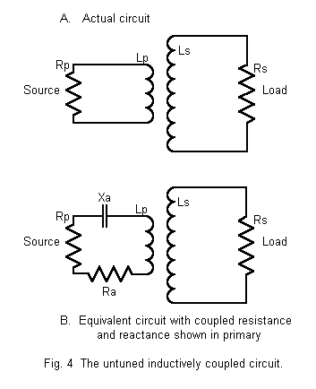


For example, suppose we use an inductor pair (taken from a table of recommended values) where LP is 1.2 micro-H and LS is 12 micro-H. XS will be 528 ohms at 7 MHz. Add a load resistance of 1500 ohms. We shall assume a coefficient of coupling (k) of 0.6. From equation (5) transformed, M = 2.3 micro-H, and the value of XM is 100 ohms. Under these conditions, using the equations above, the coupled values in the primary will be RA = 5.9 ohms and XA = 2.1 ohms.
Note that the reactance of the secondary which is coupled back to the primary is numerically equal to the transformed secondary reactance, but of the opposite sign or type. Hence, the reactances cancel in part. Ideally, selection of the right values for the two inductors and the right coefficient of coupling would provide a resistive load for the source.
In order to effect a match between the load and the source, both the mutual inductance and the reactance of one of the inductors must be varied, a highly impractical situation. I have passed along these equations only to demonstrate the reversal of reactance sign in the mutually coupled reactance, a factor that will be of importance in practical link-coupled circuits of only slightly more complex design.
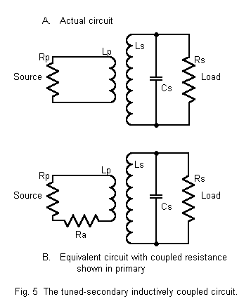
The loaded Q (QL) of the secondary of Figure 5A is given by

For loaded Qs of 10 and better, simplified equations are possible with little error. With lower values of QL, some error will results, but not outside the range of the variable components. One way to show the resistance coupled back to the primary (RA)--shown as a series resistance in Figure 5B--is with this expression:

If we use the same coil values as earlier, 1.2 micro-H and 12 micro-H, for the primary and secondary coils, along with the presumed coefficient of coupling, 0.6, we may obtain values of 100 ohms for XM and 528 ohms for XL at 7 MHz. The requisite capacitor to resonate the circuit at this frequency is 43 pF. With a load resistance of RL = 1500 ohms, QL = 2.8. Since the loaded Q of the circuit is well under 10, the calculations from this point onward will provide ballpark guidance, not accuracy, since the equations employed are intended for use with circuits with loaded Qs of 10 or more. However, employing equation (9), we derive a value for RA of about 54 ohms.
Notice that in figure 5B we have a primary impedance consisting of a resistance (desired) and a reactance (not desired in matching circuits). The reactance of the primary inductance remains uncompensated because the tuned secondary is wholly resistive. To make the primary impedance wholly resistive, we must alter the component values of the tuned circuit to permit it to show a small inductive reactance. From equation 7, we know that the transformed and coupled value of this inductive reactance will be capacitive, thus cancelling the inductive reactance. What is left will be a pure resistance.
The procedure employed is normally derived empirically rather than calculated. We tune the secondary circuit to a higher frequency than the operating frequency, normally by reducing the value of capacitance and thereby increasing the value of capacitive reactance to the increased value of the fixed inductor at this higher frequency. The parallel resonant secondary circuit at the original (slightly lower) frequency will show inductive reactance, just what we need to couple back to the primary, where it appears as a capacitive reactance in series with the reactance of the primary inductor. With the correct selection of secondary values, the primary reactances will cancel, leaving a purely resistive impedance for the primary circuit. In the process, the value of the resistance coupled back to the primary will not change by very much at all.
Because we are now using ballpark equations at low operating or loaded Qs, any calculation of this phenomenon will not be precise. However, if we walk through the process a couple of times, we can get a view of the trends and understand how things work. The standard equation for determining the reactance of a parallel combination of L and C, when transformed into reactances XL and XC for the frequency in question, is

Using the same example we have been tracking, we can plug simplified series transforms of these parallel values into equations (6) and (7) and obtain something like the values in Table 2. Although these values are not precise by any means, they do show that as we increase the resonant frequency of the parallel resonant secondary circuit, the capacitive reactance coupled back to the primary increases steadily, while the resistance decreases very slowly. The right combination of values will eventually yield a purely resistive input impedance, although the coefficient of coupling might have to be altered to keep the value of RA close to 50 ohms. Remember that in equations (6) and (7), the numerator is XM2, and raising its value will raise the values of both the RA and XA. However, the example employs a value of k of 0.6, already close to the limit of what is feasible with air-wound inductors.
Sample Values of RA and XA as the Secondary is Resonated at Higher Frequencies

Resonant    Parallel    Parallel    Series      Series      Coupled     Coupled
Frequency   Resistance  Reactance   Resistance  Reactance   Resistance  Reactance
FMHz        RL (ohms)   XP (ohms)   RS (ohms)   XS (ohms)   RA (ohms)   XA (ohms)

7.0         1500        --          186         --          54          --
7.3         1500        6590        186         42          51          -12
7.5         1500        4090        186         68          47          -18

Note 1.  Resonant Frequency refers to the resonant frequency of the parallel tuned
secondary circuit and is altered by reductions in the capacitance, while maintaining a
fixed value for the inductor.

Note 2.  Because simplified calculations have been used, the table is useful only for
noting the trends in values.  Actual values will vary considerably due both to the the
low loaded Q of the circuit and the variables of actual coupler construction.

Table 2.  Sample values of RA and XA as the secondary is resonated at higher frequencies.
The purpose of this exercise in equation-mongering is to provide you with an understanding of some of the basic principles of link-coupled tuners. More exacting forms of the equations applicable to the low values of loaded Q often encountered in ATUs are available. We have restricted ourselves to these convenient approximations because the evolution of practical coupler circuits has largely proceeded by workbench experience. If this brief account simply makes you a little more comfortable dealing with inductively coupled circuits and convinces you that they operate in accord with principles that do allow us to calculate necessary values, it will have served its purpose.
The next step is to begin wending our way through typical inductively coupled circuits in
order to see how some of the enhancements work. Unlike many other accounts of tuners, we
shall start where the transmitted signal starts: on the input side of the tuner.
Updated 11-28-97. © L. B. Cebik, W4RNL. Data may be used for
personal purposes, but may not be reproduced for publication in print or
any other medium without permission of the author.