
 Corner Reflectors Revisited
Let's begin our look at optimizing the model corner reflector further by looking at its construction, as sketched in Fig. 2 from Part 1.

The enlargement of the reflector consists in making at least one of two moves. First, one may uniformly change the length of each rod in the reflector. Second, one may add rods at 2" horizontal and vertical increments (2.8" along the 45-degree side-line).
The development of the model used in Parts 1 and 2 of this study employed only the most casual means of optimization. Changes in rod length encompassed several inches at a time until an approximate "best" length was achieved. Even though rods were added at the minimum possible rate of one per plane, the optimizing task was ended as soon as a single downturn in gain was noted. The resulting dimensions and performance were as follows (with allowance for very small numerical differences occasioned by moving the driver to a position that provides the desired feedpoint impedance.
Freq      Rod L     No. of    Side L    FS Gain   F-B Ratio Feed Impedance
MHz       inches    Rods      inches    dBi       dB        R +/- jX Ohms
432       38        14        39.6      13.60     27.27     69.7 - j 1.4
The use of this model for the comparative study rested upon several considerations. First, the modeled reflector was considerably larger than many published dimensions. Second, the model exhibited very good gain and other performance characteristics, not the least of which was the relative stability of the properties across the 420-450 MHz frequency range.
However, a number of concerns remained after working with the model. It did not achieve the maximum free space gain of 14 dBi listed in some sources. Second, the optimizing technique was sufficiently casual as to permit confusion between a gain plateau and a gain maximum. This possibility is hinted at in the gain curves in Fig. 9 by the upturn in gain at the high end of the frequency range covered by the plot.
Careful optimizing--whether manual or automated--must include sufficient tests to ensure that a gain plateau followed by a gain drop is not interpreted automatically as having passed the point of maximum gain for an array. Several systematic increments of dimensional change must follow the detection of maximum gain to give confidence in the peak figure. Alternatively--as found in some genetic optimizing routines--one can use a method of "jumping" over regions of decreased gain to see if there is a different geometry that produces an even higher gain.
Therefore, let's return to the model and see if further optimizing is possible. After an initial "jump" in dimensions, we shall look very closely at small changes in gain. Optimizing is one of those modeling enterprises in which it makes sense to carry out reported values to whatever number of decimal places it takes to see a difference, even if operationally, a particular change may seem to make no difference.
(Those who insist upon reducing all gain and other NEC output figure uniformly to integers or other units that make operational differences may in fact be missing an entire dimension of what NEC makes available when used analytically. The level of precision that may be spurious to operational considerations can be vital wherever numerical trends make a difference to a design or analysis project. On the other hand, suggesting that the antenna which I built in my garage has a gain of 13.783 dBi would only make sense as an exercise in humorous hyperbole.)
The present task is to see if the gain of a corner reflector can be raised to about 14 dBi free space at 432 MHz, the design frequency. An added constraint is that the gain must be reasonably stable between 420 and 450 MHz.
We may set aside several potentially complicating factors with the following notes. First, the changes to be made to the reflector planes in terms of the number of rods and their length have no significant effect upon the feedpoint impedance when the driver is left in the positions noted in Part 2 for 50, 70, and 100 Ohms feedpoint impedance. Even when surveyed across the band, the SWR limits remained very tightly matched to the figures given in Part 2, with changes only in the hundredth's column. Once the horizontal dimension of the corner array is considerably more than double the distance from the driver to the reflector apex, source impedance appears to remain very stable.
Second, the front-to-back figures for all models showed a minimum 180- degree ratio of 25 dB. Therefore, variations in these figures were considered insignificant for the present enterprise. Related to this feature is the fact that the pattern shape also remained stable, with -3 dB beamwidths in the 36-40 degree range throughout. Hence, the shapes shown in Part 1 of this exercise remain good indicators of the patterns derived from further optimizing efforts.
Throughout, the basic model structure has been retained, including the use of 3/8" diameter aluminum tubing for all elements of the corner reflector, including the driver. Hence, the optimizing efforts are valid only for this structure. The use of smaller or larger diameters of reflector rods may require re-optimizing the model. nonetheless, within this limits, we may focus our attention to the gain patterns yielded by the model with different rod lengths and different numbers of rods.
A gain peak emerges as the side length of the reflector planes approaches 2 wl. Therefore, optimizing efforts were concentrated in this region, using (without counting the apex rod) 19, 20, and 21 rods for side lengths of 53.7" (1.97 wl), 56.6" (2.07 wl), and 59.4" (2.17 wl at 432 MHz). This spread represents about a 10% overall change of side length for the reflector planes. For each of the side length options, I looked at rod lengths of 36, 37, and 38 inches.
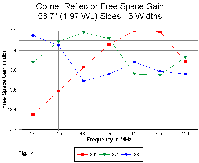
The first gain curve (Fig. 14) is for 19 rods. Immediately apparent is that the curve for the 37" rod length yields a curve whose shape is similar to the one shown in Part 2, with a peak near the design frequency, a gain decrease above that frequency, and a final upturn at the highest frequency tested. Use care in interpreting steep curves, since the range of gain for the entire graph is 1 dB.
Of equal importance are the other two curves. In fact, they show a frequency displacement of relatively similar curves. The curve for the 36" rods shows its peak higher in the passband. The curve for the 38" rods moves the gain decrease region lower in the passband to encompass the design frequency.
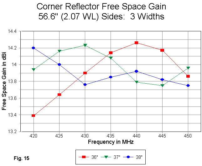
When each reflector plane is lengthened by one rod (2.8"), we obtain the curves in Fig 15. They are quite similar to those in the preceding graphic, but with slightly higher gain peaks for all three curves. The fact that the curves are being displaced slightly lower in frequency (relative to the preceding graph) is almost invisible.
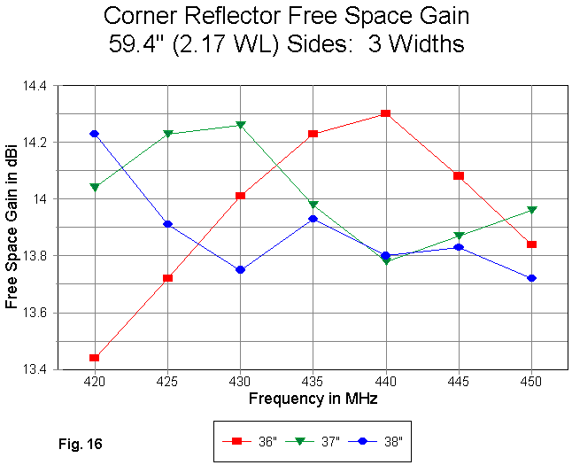
Increasing the reflector plane to 21 rods and 59.4" yields Fig. 16. By this time, the lowering of the curves in frequency with increases in reflector length is more readily apparent. Also apparent is the fact that the 37" rod length--for the overall structure under study--is closest to optimal for achieving the maximum gain at the design frequency and the most even gain across the frequency span covered.
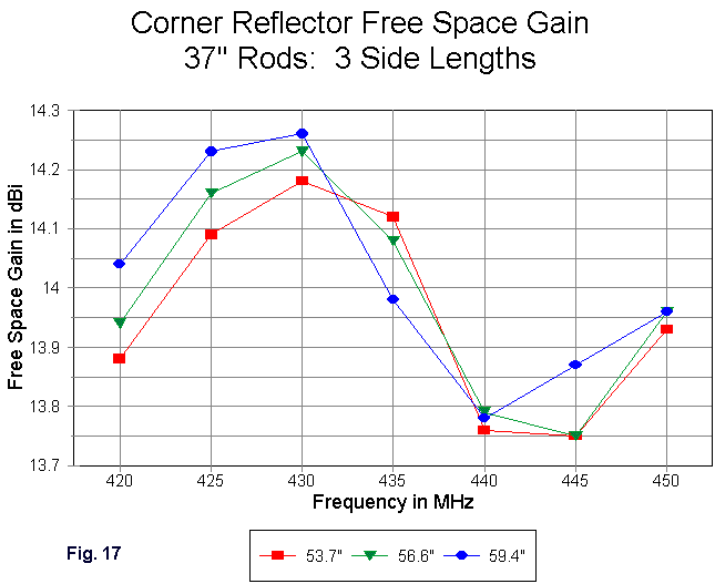
Fig. 17 combines the gain curves for the 37" rod lengths for a comparison of the three side lengths. The peak free space gain of the longest reflector exceeds 14.25 dBi. However, the true peak is below 430 MHz, and the curve is on a downward trend, so that the 432 MHz gain of the intermediate reflector actually numerically exceeds it.
However, a new trend is also appearing. In the models in Part 2, the maximum differential between a gain peak and null was under 0.4 dB. The differential at the new longer reflector side length begins to exceed 0.5 dB. Even if more gain is obtainable with further increases in the side length of the reflectors, it may be purchased at the cost of smooth gain response across the frequency spread of interest.
One might continue the progression of optimizing studies further, especially if one is interested in a particular frequency of operation. further adjustment of reflector rod length and reflector side length may yield perhaps another 0.2 dB of gain increase. However, due to the increasing size of the models involved, I decided to stop at this point.
Let's compare the result of this exercise with the model with which we began.
Freq      Rod L     No. of    Side L    FS Gain   F-B Ratio Feed Impedance
MHz       inches    Rods      inches    dBi       dB        R +/- jX Ohms
432       38        14        39.6      13.60     27.27     69.7 - j 1.4
432       37        20        56.6      14.21     29.23     70.2 - j 1.4
We have gained 0.6 dB gain. Before we end the optimization exercise, we should ask, "At what cost?"
Finding the maximum gain peak and then setting it right on 432 MHz might require a very precise rod length. For those so inclined, a length just below 37" will move the curves upward in frequency. Each side length will require a unique rod length. This fact has implications for physically implementing the design using real materials. When modeled dimensions become too finicky, it does not bode well for constructing an antenna that matches the model in performance, since numerous construction variables may intervene.
Apart from this question, the general size of the corner reflector has significantly increased with the addition of 5 to 7 new reflector rods. Fig. 18 indicates the approximate growth, using the intermediate optimized model in comparison with the model used in Parts 1 and 2.
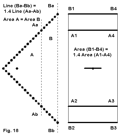
Interestingly, the side length has increased by a factor of about 1.4, which results in an aperture increase of the same amount. There is a weight increase of about 40%. More importantly, the area encompassed by the side dimensions has doubled. The implications for balance, weight, wind loading, and other factors affected by the larger structure should be immediately apparent. Moreover, maintaining precision construction over the larger structure--and over the lifetime of the structure in service-- also become a factor in deciding whether or not to go for maximum possible gain.
Moreover, the 0.6 dB gain does not accumulate in stacks of corner reflectors. It is rather a one-time gain that may in fact increase the overall physical difficulty of implementing the entire stack.
Nonetheless, the exercise has been far from idle. When combined with the models used in Parts 1 and 2, the new work suggests that there is a degree of periodicalness in gain vs. reflector structure. Hence, reflector plane size is not a matter of arbitrary selection once certain limits have been observed. Instead, the development of corner reflector designs deserves all of the detailed attention we give to other antenna types. Modeling, while limited in some respects, can be useful with this class of antennas. However, there are material selections that may require careful field testing to obtain precisely the right dimensions for the reflector planes so that the antenna provides--at any size--all of the performance of which it is capable.
Corner refl + dipole: 432 MHz           Frequency = 432  MHz.

Wire Loss: Aluminum -- Resistivity = 4E-08 ohm-m, Rel. Perm. = 1

              --------------- WIRES ---------------

Wire Conn. --- End 1 (x,y,z : in)  Conn. --- End 2 (x,y,z : in)   Dia(in) Segs

1           -5.660,  9.600,  0.000         5.660,  9.600,  0.000 3.75E-01  11
2          -18.500,  0.000,  0.000        18.500,  0.000,  0.000 3.75E-01  31
3          -18.500,  2.000,  2.000        18.500,  2.000,  2.000 3.75E-01  31
4          -18.500,  4.000,  4.000        18.500,  4.000,  4.000 3.75E-01  31
5          -18.500,  6.000,  6.000        18.500,  6.000,  6.000 3.75E-01  31
6          -18.500,  8.000,  8.000        18.500,  8.000,  8.000 3.75E-01  31
7          -18.500, 10.000, 10.000        18.500, 10.000, 10.000 3.75E-01  31
8          -18.500, 12.000, 12.000        18.500, 12.000, 12.000 3.75E-01  31
9          -18.500, 14.000, 14.000        18.500, 14.000, 14.000 3.75E-01  31
10         -18.500, 16.000, 16.000        18.500, 16.000, 16.000 3.75E-01  31
11         -18.500, 18.000, 18.000        18.500, 18.000, 18.000 3.75E-01  31
12         -18.500, 20.000, 20.000        18.500, 20.000, 20.000 3.75E-01  31
13         -18.500, 22.000, 22.000        18.500, 22.000, 22.000 3.75E-01  31
14         -18.500, 24.000, 24.000        18.500, 24.000, 24.000 3.75E-01  31
15         -18.500, 26.000, 26.000        18.500, 26.000, 26.000 3.75E-01  31
16         -18.500, 28.000, 28.000        18.500, 28.000, 28.000 3.75E-01  31
17         -18.500, 30.000, 30.000        18.500, 30.000, 30.000 3.75E-01  31
18         -18.500, 32.000, 32.000        18.500, 32.000, 32.000 3.75E-01  31
19         -18.500, 34.000, 34.000        18.500, 34.000, 34.000 3.75E-01  31
20         -18.500, 36.000, 36.000        18.500, 36.000, 36.000 3.75E-01  31
21         -18.500, 38.000, 38.000        18.500, 38.000, 38.000 3.75E-01  31
22         -18.500, 40.000, 40.000        18.500, 40.000, 40.000 3.75E-01  31
23         -18.500,  2.000, -2.000        18.500,  2.000, -2.000 3.75E-01  31
24         -18.500,  4.000, -4.000        18.500,  4.000, -4.000 3.75E-01  31
25         -18.500,  6.000, -6.000        18.500,  6.000, -6.000 3.75E-01  31
26         -18.500,  8.000, -8.000        18.500,  8.000, -8.000 3.75E-01  31
27         -18.500, 10.000,-10.000        18.500, 10.000,-10.000 3.75E-01  31
28         -18.500, 12.000,-12.000        18.500, 12.000,-12.000 3.75E-01  31
29         -18.500, 14.000,-14.000        18.500, 14.000,-14.000 3.75E-01  31
30         -18.500, 16.000,-16.000        18.500, 16.000,-16.000 3.75E-01  31
31         -18.500, 18.000,-18.000        18.500, 18.000,-18.000 3.75E-01  31
32         -18.500, 20.000,-20.000        18.500, 20.000,-20.000 3.75E-01  31
33         -18.500, 22.000,-22.000        18.500, 22.000,-22.000 3.75E-01  31
34         -18.500, 24.000,-24.000        18.500, 24.000,-24.000 3.75E-01  31
35         -18.500, 26.000,-26.000        18.500, 26.000,-26.000 3.75E-01  31
36         -18.500, 28.000,-28.000        18.500, 28.000,-28.000 3.75E-01  31
37         -18.500, 30.000,-30.000        18.500, 30.000,-30.000 3.75E-01  31
38         -18.500, 32.000,-32.000        18.500, 32.000,-32.000 3.75E-01  31
39         -18.500, 34.000,-34.000        18.500, 34.000,-34.000 3.75E-01  31
40         -18.500, 36.000,-36.000        18.500, 36.000,-36.000 3.75E-01  31
41         -18.500, 38.000,-38.000        18.500, 38.000,-38.000 3.75E-01  31
42         -18.500, 40.000,-40.000        18.500, 40.000,-40.000 3.75E-01  31

              -------------- SOURCES --------------

Source    Wire      Wire #/Pct From End 1    Ampl.(V, A)  Phase(Deg.)  Type
          Seg.     Actual      (Specified)

1           6     1 / 50.00   (  1 / 50.00)      1.000       0.000       V
Updated 4-18-99. © L. B. Cebik, W4RNL. Data may be used for personal purposes, but may not be reproduced for publication in print or any other medium without permission of the author.