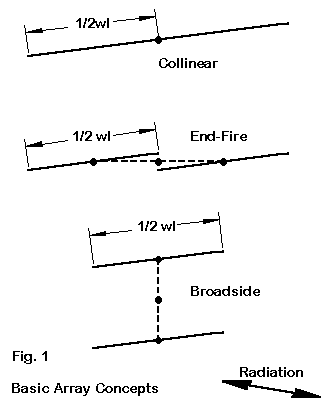
Figure 1 shows three basic arrangements that yield the fundamental categories within which these arrays are specified. Elements are collinear when they are arranged end-to-end so that the main radiation lobes are tangential to the wire. The ends may touch, as in the illustration, or they may be separated by a phasing section, a length of wire or transmission line that alters the current phase and magnitude at the point of junction. Ordinarily, these lines are used to increase the strength of the main radiation lobes.
When elements are parallel to each other, in a plane that is parallel to the ground surface, and the strongest radiation lobes are tangential to the wires, we have an End-Fire array. Most commonly for bi-directional arrays, the two elements are fed 180 degrees out of phase with each other.
A Broadside array places elements (normally) in a vertical plane, with the main radiation lobe again tangential to the wires. In this configuration, we feed the wire elements in phase with each other.
Most bi-directional wire arrays use combinations of these techniques. For most applications, a 1 wl wire is the shortest collinear element having sufficient gain to use in either a broadside or end-fire array. Longer elements, such as the 1.25 wl extended double Zepp (EDZ), are commonplace. Moreover, we may combine both end-fire and broadside techniques into single arrays. For many of the bi-directional array designs, absolute precision of wire length is less important than with other types of antennas. A 5% variation in the length of a 1/2 wl element may make little difference to the performance of the array. Indeed, as arrays grow larger, modeling does not so much determine an exact construction version as it looks at trends in both performance and source impedance to guide field adjustment of the physical antenna. In addition, we should not expect source impedances that are ready matches to a 50-Ohm system feedline. Instead, we shall find a wide variety of source impedances that challenge us to develop feed networks.
Although bi-directional arrays date from the earliest days of radio communications, they reached a zenith of design effort in the 1930s as short wave broadcasting became commonplace. Great "antenna farms" involving acres of land emerged as stations built multiple fixed-position antennas beaming power with narrow beamwidths at selected reception areas. Although new ideas in bi-directional arrays surface more slowly today, designing an antenna of this type to serve a specific communications need is still a significant engineering enterprise.
In some applications, especially in the upper HF range, the Yagi and other rotatable parasitic antennas have supplanted the bi-directional array. However, up to about 10 MHz, the bi-directional array is still the antenna of choice for most fixed stations. Moreover, even above 10 MHz, these antennas offer a cost-benefit ratio that make them attractive alternatives to other techniques.

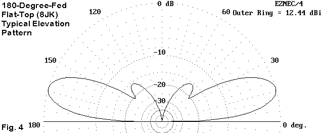
Figure 2 shows the top view of a flat-top or 8JK and a broadside view of a Lazy-H.
Virtually all flat-top arrays of 2 elements are fed 180-degrees out of phase. The simplest means of achieving this goal is to create two transmission lines of equal length to an added central source wire (junction). One line is reverse connected to its element. Since the current magnitude and phase shift along each line is identical, the reverse connection on one of the lines ensures the out-of-phase condition.
Virtually all vertically-stacked 2-wire arrays are fed in-phase. Once more, the simplest feed system is to use equal lengths of transmission line to an added common junction wire, but normal connections are used for both lines. Ordinarily, the slight differences in the source impedance of the two wires, given their different distances from the earth's surface, is not sufficient to disturb the relative phasing. However, in very sensitive systems, networks may be used to achieve critical phasing adjustments.

For all arrays, it is best to develop models in step-wise fashion, rather than throwing together all the elements and then wondering what might be wrong with the overall result. Figure 3 shows the steps.
1. First, create the wires and use a separate source for each. With the simple expedient of alternately feeding one wire 180 degrees out of phase with the other wire and then in phase, you will see the pattern results appropriate to your design. You will also have a record of the wire source impedances, should you decide to do some independent calculations for a feed system.
2. Next, try the most direct feed system possible. This step involves creating a very short, thin wire in the model physically located exactly between the two antenna wires and along the center line of those elements. If you are using NEC-2, you can create two transmission lines, one from each antenna wire to the common or junction wire. Place the source on this third wire (remembering to remove the two formerly independent sources). Use the connections appropriate to the antenna type.
Record the composite source impedance. The key question at this point is whether that impedance is acceptable in terms of the system feed from that point back to the transmitting/receiving equipment. Within the scope of this step, you have the option of changing the characteristic impedance of the line, most usually within the 300/450/600 Ohm set of commercially available transmission lines. However, you can always construct your own.
Be certain to allow for the velocity factor (VF) of the line. Some programs permit direct entry of this value; others require that you precalculate the longer line length with a VF of 1.0 equivalent to a direct connection with a lines whose VF is less than 1.0.
In some cases, you will be "stuck" with the composite source impedance that emerges. Often, the direct line feed is the only physically feasible system of routing the feedlines. In some other cases, you may have the option of running longer lines to a common junction point.
3. If you can manage longer lines, you may experiment with them to see if they yield a more desirable composite source impedance than direct feed.
The following table illustrates the process, using a 1/2 wl spaced flat-top with 180-degree out-of-phase feeding. The frequency is 14.175 MHz, resulting in each line having a minimum length of about 17.5 feet.
Line length              Composite source impedance
(each leg)          600-Ohm line             450-Ohm line
 17.5'               44.4 - j  4.4            25.0 - j  1.7
 20.0'               46.5 + j 63              26.2 + j 50
 22.5'               54.1 + j137              30.7 + j106
 25.0'               71.3 + j228              40.7 + j176
 30.0'              216   + j556             129   + j444
For a coax match, the most direct feed with 600-Ohm coax seems best. However, other feed systems may direct the use of other lengths. While you are at it, do a frequency sweep of the antenna to check the rate of change of both the resistive and reactive components of the composite source impedance. You may also change the wire lengths to place the resonant point of the system at a different resistive value of impedance.
On the other hand, in-phase fed broadside systems, such as the Lazy-H, often permit multi-band service with usable gain and patterns extending from 0.5 F to 1.25 F, where F is the frequency for which each element is 2 half-wavelengths. Consider the Lazy-H cut for about 21 MHz, with 44' wires spaced vertically by 22' (about 1/2 wl). If the lower wire is at 35' up, the upper wire will be 57' high. (This system might also be called an EDZ Lazy-H cut for 28 MHz and spaced about 5/8 wl at that frequency.) The following table records the modeled performance on various amateur frequencies.
Frequency      T-O Angle      Gain dBi       Source Impedance
10.1           28              7.38           50 + j  91
14.0           20              9.04          572 - j 394
18.1           16             10.56           49 - j 142
21.0           13             12.15           24 - j  36
24.9           11             14.31           17 + j  94
28.0           10             14.78           39 + j 291
If the source impedances are not an issue, this antenna might be useful as a multi-band antenna serving 30 through 10 meters with minimally dipole performance at the lowest frequency. You may verify that all patterns are broadside to the antenna, in contrast to the many-lobed patterns that would appear on 10 meters had we started with a 30-meter dipole. You may also wish to experiment with other line lengths from the center source junction to the antenna elements to see if you can arrive at a length more favorable to your own feed system ideas.
With phasing lines and NEC-2 we always have 2 options, as shown in Figure 5, a representation of collinear EDZ antenna elements. (Of course, only the physical modeling option is open to those who use MININEC. However, it is the initial option of choice for all modeling.)
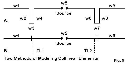
Only some types of arrays are amenable to the substitution of non-radiating transmission-line models for their stub elements. A few depend upon the incomplete cancellation of currents to yield their final performance figures. Therefore, it is usually wise to begin with a physical model of a collinear element and ten later to convert it to a transmission line model.
Physical modeling is straight forward, as the figure indicates. All wires should run continuously, from end 1 of wire 1 to end 2 of wire 9. Use a segmentation density high enough that the horizontal shorting lines of the stubs are not radically different in length from the wire segments immediately adjacent to them. In developing the model, make use of either the current tables or a graphical aid to show relative current magnitudes. See Figure 6.
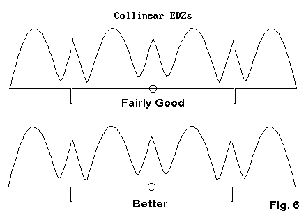
The aim of the collinear EDZ design is to place equal magnitude currents at each of the phasing lines. Unequal currents result in radiation from the phasing lines, which can disrupt overall performance. The current magnitude graphics represent two stages on the way to perfecting a model of the antenna in question.
This design, which dates back to the 1930s work of Hugo Romander, W2NB, is actually fairly forgiving, with 2-3% errors in length yielding only a drop of a few tenths of a dB in gain. The beamwidth of this antenna is only about 17 degrees between -3 dB points, so it is best suited to point-to- point communications rather than casual amateur work.
Wide-spaced physical stubs do not change their length rapidly as they are made narrower, since the characteristic impedance of these shorted stubs changes slowly as the spacing is increased beyond a couple of inches. Therefore, they provide a starting point for replacement with transmission line sections. The easiest procedure in many cases is to use 600-Ohm line for initial replacement trials. Once a working length value is found, you may convert it to an inductive reactance and from there to any transmission line value with a length appropriate to its characteristic impedance and velocity factor. Place the transmission line stubs on the first and last segment of the center wire (relative to the model in Figure 6), and use a segmentation density high enough to closely approximate the center wire ends.

Figure 7 shows a side view of a Sterba curtain, similar to the typical sketch shown in many an antenna manual. The twisted vertical line pairs seem to beg for transmission line treatment. If we contemplate using physical lines, we often bog down in the thought of trying to keep them at a constant spacing and still effecting the "half-twist."
The top view shows a simple solution. Offset two wires by a small space. 0.5' will do at 40 meters without creating the slightest distortion in antenna performance for this 2.5 wl antenna. Run one wire from end to end, using vertical lengths to let it alternate between the top and bottom positions. Run the other wire the same way, but start at the far end and opposite corner. The result will be a set of wires correctly oriented to each other in both the horizontal and vertical planes. Connect the near and far ends with "near-vertical" wires (offset from the vertical only by the space between the horizontals). Make the connections to keep the wire continuous from its start to finish.
Here is a typical table of wires, with the wire offset in the Y-axis.
Sterba curtain:  Frequency = 7.2  MHz.
Wire Conn.--- End 1 (x,y,z : ft)  Conn.--- End 2 (x,y,z : ft) Dia(in) Segs

1   W20E2   0.000,  0.500, 67.000  W2E1   0.000,  0.000,134.000  # 12   15
2    W1E2   0.000,  0.000,134.000  W3E1  33.500,  0.000,134.000  # 12    8
3    W2E2  33.500,  0.000,134.000  W4E1  33.500,  0.000, 67.000  # 12   15
4    W3E2  33.500,  0.000, 67.000  W5E1 100.500,  0.000, 67.000  # 12   15
5   W21E1 100.500,  0.000, 67.000  W6E1 100.500,  0.000,134.000  # 12   15
6    W5E2 100.500,  0.000,134.000  W7E1 167.500,  0.000,134.000  # 12   15
7    W6E2 167.500,  0.000,134.000  W8E1 167.500,  0.000, 67.000  # 12   15
8    W7E2 167.500,  0.000, 67.000  W9E1 234.500,  0.000, 67.000  # 12   15
9    W8E2 234.500,  0.000, 67.000 W10E1 234.500,  0.000,134.000  # 12   15
10   W9E2 234.500,  0.000,134.000 W11E1 268.000,  0.000,134.000  # 12    8
11  W10E2 268.000,  0.000,134.000 W12E1 268.000,  0.000, 67.000  # 12   15
12  W11E2 268.000,  0.000, 67.000 W13E1 234.500,  0.500, 67.000  # 12    8
13  W12E2 234.500,  0.500, 67.000 W14E1 234.500,  0.500,134.000  # 12   15
14  W13E2 234.500,  0.500,134.000 W15E1 167.500,  0.500,134.000  # 12   15
15  W14E2 167.500,  0.500,134.000 W16E1 167.500,  0.500, 67.000  # 12   15
16  W15E2 167.500,  0.500, 67.000 W17E1 100.500,  0.500, 67.000  # 12   15
17  W21E2 100.500,  0.500, 67.000 W18E1 100.500,  0.500,134.000  # 12   15
18  W17E2 100.500,  0.500,134.000 W19E1  33.500,  0.500,134.000  # 12   15
19  W18E2  33.500,  0.500,134.000 W20E1  33.500,  0.500, 67.000  # 12   15
20  W19E2  33.500,  0.500, 67.000  W1E1   0.000,  0.500, 67.000  # 12    8
21   W4E2 100.500,  0.000, 67.000 W16E2 100.500,  0.500, 67.000  # 12    1
For this particular model, the source is placed in wire 21, which corresponds to the alternate source point. You may omit wire 21 and employ a split feed system, using the last segment on wire 20 and the first segment on wire 1 as the source positions. There are minor differences in current equality on the horizontal sections between the two sourcing systems, as you may see from the current tables or the graphical current magnitude facility in your program. These differences will alter the gain slightly and also the degree to which the 26-degree beamwidth main lobe is offset from being directly broadside to the wire array. However, the source impedance at the end position may be more convenient, being closer to 600 Ohms. You may undertake many modeling experiments, especially with the vertical spacing between the top and bottom wires of the system, to effect the most equal current distribution possible.
If these notes have a message, it is something like this: model slowly and progressively toward the final complete antenna package (to the degree that your program permits modeling it). Double check all input values before running the model at each stage. Along the way, make use of all of the data provided by the program (and not just gain and source impedance results) to perfect the model.
The more we learn about using the vast array of data provided by antenna
modeling programs, the better--and quicker--and more informative our models
become.