The chief sources of commercial implementations of NEC-2 are the following:
NEC-Win programs are for Windows 95, while NEC-Wires and EZNEC are DOS-based programs.
The basic reference for NEC-2 is J. Burke, A. J. Pogio, "Numerical Electromagnetic Code (NEC) Method of Moments, a User Oriented Code," Vol. 2 (Part III: User's Guide), Tech. Doc. 116, Naval Systems Center, San Diego, 1982. For those desiring to create their own input and output systems, NEC-2 is public domain and available in FORTRAN and compiled versions. Ray Anderson, WB6TPU, maintains a site for downloading basic NEC-2 materials: URL: http://www.qsl.net/wb6tpu
Segment length should be under 0.1 wavelength long, with 0.05 wavelength preferred (about 10-11 segments per half-wavelength). Segments shorter than 0.001 wavelength should also be avoided. For reference, the following table provides a ham band list of the maximum and minimum recommended segments lengths.
Frequency      Segment Length in inches    Shortest Segment
               for 0.05 wl segments        Length in inches
1.8                 327.9                    6.657
3.5                 168.6                    3.372
7.0                  84.3                    1.686
10.1                 58.4                    1.169
14.0                 42.2                    0.843
18.068               32.7                    0.653
21.0                 28.1                    0.562
24.89                23.7                    0.474
28.0                 21.1                    0.422
50.0                 11.8                    0.236
144.0                 4.1                    0.082
Thin-wire segments are preferred: as with MININEC, the wire circumference divided by the wavelength should be much less than 1 for accurate results. Moreover, the ratio of segment length to diameter should be greater than 4 for errors less than 1%. If the model demands a smaller ratio, it should be approached cautiously by shortening segment lengths gradually with an eye toward results taking off on a tangent.
Maintaining a larger segment length to diameter ratio at corners is also necessary to keep the center of one segment from falling within the radius of the other segment. Again, approaching this limit produces nothing sudden, so that it can be pressed, but cautiously.
Unlike MININEC, angled antenna elements do not require special treatment other than the warning about very short segment-length-to-wire-diameter ratios. NEC-2 will model equally segmented wires in a quad quite handily.
However, prevent wires from physically touching or coming in very close proximity when crossing. There is no hard and fast rule on where the proximity limits occurs, but separation by several wire diameters is recommended.
Another NEC-2 limitation is the inability to model small loops, less the about 0.1 wavelength in circumference.
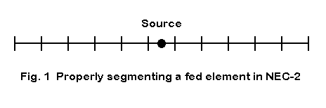
NEC-2 documentation specifically recommends that closely space parallel wires be arranged so that the segments are carefully matched, as shown in Figure 2. As noted in the last episode, this practice is a good one to follow with all models.

The second junction limitation concerns feeding multiple antennas at a common source point. This problems differs from feeding a single bent element (such as inverted Vee) at the apex. In this case, the modeler can often use a split feed, feeding with separate sources the segments on each side of the wire junction. If the segments are short, the resulting sum of the two impedances will yield an accurate overall source impedance for the antenna. Some programs provide for a split voltage or current feed and report the source conditions (voltage, current, and impedance) as a single set of values.
When multiple antenna elements join at a single point, it is no longer possible to employ a split feed effectively. The simplest case is the spread dipole for two bands with a single feedpoint, as shown in Figure 3.
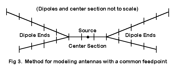
The simple work-around is also shown in Figure 3: adding a small common section of wire for the source and joining the diverging elements to the ends of this wire. Recommendations for this segments include a minimum length of 0.02 wavelength and 3 segments. Equally important, the adjoining segments of the diverging wires should be about the same length as those in the center section.
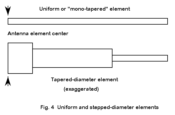
If an element is comstructed on each side of center by, say, only 2 wires of different diameters and the junction of these wires is past the mid-point on each side, modeled results will be more accurate than with elements having multiple diameter steps closer to the center. Large steps in diameter also increase the accuracy problem.
Most commercial implementations of NEC-2 have incorporated a technique to overcome this problem effectively. Using equations developed by Dr. David Leeson, the programs calculate the antenna properties with substitute elements having a constant diameter. The resulting models have proven quite reliable. However, you must use caution in constructing the model to ensure that the stepped diameter element is continuous or collinear, with no bends or intervening geometric oddities along the way. For example, adding a mid-element capacity hat structure will disable the correction feature in some programs. Likewise, the source must be at the center of an element with open ends (such as a dipole), and loads must be symmetrically placed. Transmission line are sometimes disallowed. Moreover, the element may be required to be within a certain percentage of resonance, which may complicate attempts to model in NEC-2 multi-band HF Yagis with stepped-diameter elements throughout.
Let's take a closer look at the effects of using and not using the substitute elements in place of the stepped diameter elements. The following table shows several aluminum dipole elements for 14 MHz, ranging from a uniform 1" wire to a highly stepped set of wires. Lengths and diameters are from the end to center, with the other side symmetrical to the given side. Except for the uniform element, NEC-2 outputs are shown for both the substitute and the uncorrected elements.
Length(s) from center in inches     Free Space Gain    Source Impedance
  Diameter(s) in inches                 in dBi         (R +/- jX Ohms)
1.  Uniform element (no corrective needed)
     -201.25...0                         2.12            71.8 - j 0.6
            1.0
2.  One step, far out
     -204...-150...0       No Cor.       2.14            73.0 + j 4.4
        0.75    1.0
     -201.45...0           Cor.          2.12            72.0 + j 0.4
          0.966
3.  One step, near center
     -204...-50...0        No Cor.       2.22            72.4 + j 5.2
        0.75   1.0
     -201.661...0          Cor.          2.13            71.8 - j 0.5
           0.792
4.  Two steps, modest taper
-205.75...-100...-20...0   No Cor.       2.32            72.5 + j10.6
      0.75    1.0  1.25
-201.49...0                Cor.          2.13            71.9 + j 0.1
     0.889
5.  Two steps, more extreme taper
-208.5...-100...-20...0    No Cor.       2.82            67.6 + j17.1
     0.75    1.0   2.5
-201.63...0                Cor.          2.13            72.1 + j 0.9
     0.895
The corrected substitute models ("Cor.") are those generated by the program as replacement elements for the original model, which reflects the intended tapered diameter structure. With only moderate levels of diameter stepping, uncorrected NEC-2 reports of gain rapidly become unreliably large, while source impedances improperly show the elements to be too long relative to resonance.

Consider the single quad loops in Figure 5. If we construct such a loop for 28.5 MHz of #14 wire, then about 9.13' of wire per side (1041/f) will yield a loop with a free space gain of about 3.24 dBi and a source impedance of 126-127 Ohms resistive. This is true whether we model the antenna as a fully length-tapered MININEC item or as a NEC-2 wire antenna with reasonable segmentation. If we make the element 1" in diameter, then 9.5' per side (1083/f) in both programs yields a gain of about 3.4 dBi with a resonant source impedance close to 132 Ohms.
However, if we change the construction so that the horizontal portions are "fat" while keeping the vertical portions of "thin" wire, the results are far different. The following table shows how.
Antenna Dimensions                 Free Space Gain     Source Impedance
                                        dBi            (R+/-jX Ohms)

1.  0.5" dia hor/#12 vert:  10.15' per side
     MININEC tapered                    3.61           136.7 - j 2.3
     NEC-2                              3.57           175.4 + j140
2.  1.0" dia hor/#14 vert:  10.7' per side
     MININEC tapered                    3.80           141.6 - j 5.7
3.  1.0" dia hor/#14 vert:  9.68' per side
     NEC-2                              3.46           138.4 - j 0.5
The first antenna uses the same model in both programs. Compared to the materials of antennas 2 and 3, this model has a less extreme difference in wire diameters between the horizontal and vertical portions. Although the gain figures produced are close, the source impedance are radically different, as NEC-2 suggests a far smaller loop size for resonance.
Antennas 2. and 3. use a larger difference between the horizontal and vertical wire diameters. The two models use the same horizontal to vertical wire diameter ratios, and each is each brought close to resonance. Although the source impedances are now comparable between MININEC and NEC- 2, the loop sizes for resonance are very far apart.
Divergent results of this order require empirical verification before either modeling system can be trusted for dissimilar diameter materials meeting at the corners of an antenna element. So I modeled a 50-Ohm fat-horizontal, thin-vertical wire loop for 146 MHz. The 0.75" diameter horizontal bars were 16" long. For resonance, NEC-2 called for 29.15" #14 (0.064" diameter) vertical wires, while NEC-4 called for 32.2" wires. Uncorrected MININEC resonated the loop with 33.7" vertical wires. The test antenna resonated with 33.75" vertical wires. The real antenna result can be up to about +/- 3/8" in error due to possible variances from the model created by screw heads and short leads to the antenna coax fitting. However, the dimensions are sufficiently accurate to demonstrate the greater reliability of MININEC results and the problems of modeling corner junctions of dissimilar diameter wires in NEC-4 and NEC-2.
An interesting deviation from this pattern occurs when right-angle junctions of dissimilar diameter wires involve symmetrical arrangements of one size of the wires. These models include vertical antennas with elevated ground radial systems, dipoles or verticals with "capacity hats," and similar structures. In these cases, the apparent cancellation of radiation from the elements of the symmetrical portion of the structure yields accurate gain and source impedance reports. A series of experimental models, verified by measurements with antennas built from the models, showed an agreement between NEC-2 and MININEC models within 1 to 2 percent for the radial length in capacity hats on 10-meter dipoles and 2-element Yagis.

Folded dipoles using dissimilar diameter wires add another dimension to the NEC-2 limitations. Consider two folded dipoles, as shown in Figure 6. One consists of 2 parallel wires 0.5" in diameter spaced 0.25' apart and 16.1' long for 28.5 MHz. The other consists of one 0.5" diameter wire and one #12 (0.808" diameter) wire, also 0.25' apart and 16.2' long for 28.5 MHz. The results of modeling these antennas in both MININEC and NEC-2 are as follows:
Antenna Dimensions                 Free Space Gain     Source Impedance
                                        dBi            (R+/-jX Ohms)

1.  2 x 0.5" dia; 16.1' long
     MININEC                            2.22           285.7 + j 0.9
     NEC-2                              2.22           285.9 + j 4.1
2.  0.5" dia and #12; 16.2' long
     MININEC                            2.21           530.5 + j 1.5
     NEC-2                              0.69           375.2 + j25.8
Both systems model the standard folded dipole with very reasonable accuracy. The second, non-standard, folded dipole with dissimilar wire diameters is another matter. Standard textbook equations for calculating the impedance of folded dipoles with dissimilar diameters yield a projected ratio for the source impedance of the folded dipole relative to a single-wire dipole of nearly 7.5:1, or between 530 and 535 Ohms. While the MININEC model falls in the ball park (considering that the formula does not account for antenna shortening or end connections between the two wires), the NEC- 2 model is clearly unusable.
The end result of exploring these limitations is this: wherever NEC-2 is to be used with wire junctions or closely spaced wires of dissimilar diameters, extreme caution must be used to independently check the reliability of the reported performance specifications.
The contrast between the results of the MININEC ground system and the S-N system are sufficiently vivid with low dipoles, that I shall repeat a table presented in the last episode. The following table compares NEC-2 (S-N) and MININEC data for a 3.5 MHz dipole (resonated in free space) at heights from 0.05 to 0.30 wavelengths above medium or "average" earth (conductivity = 0.005 Siemans/meter; dielectric constant = 13).
                         MININEC                  NEC-2 (S-N Ground)
Antenna                  137.2' #12 copper        136.9' #12 copper
Height                   Gain      Source Z       Gain      Source Z
 W/L      Feet           dBi       R +/- jX       dBi       R +/- jX
0.05      14.05          9.4        7.4 - j 4.9   1.2       48.9 + j15.4
0.10      28.10          8.4       23.3 + j20.5   5.1       49.8 + j21.1
0.15      42.15          7.7       45.9 + j35.1   6.4       62.5 + j26.9
0.20      56.20          7.0       62.3 + j37.0   6.5       77.0 + j25.3
0.25      70.26          6.2       87.7 + j28.3   6.2       87.8 + j17.3
0.30      84.31          5.9       97.4 + j13.5   6.1       92.3 + j 6.1
Despite the clearly more reliable figures produce in NEC-2, the use of the S-N is not without some limitations. For example, NEC-2 is sometimes used to simulate surface ground radial systems with vertical antennas by placing the radial wires very close to the ground. One recommendation sets the minimum height at 0.0001 wavelength, with segment-length tapering techniques applied between that height up to 0.001 wavelength. For frequencies below the 80-meter ham band, some ground-wave measurements suggest that elevated radial models yield overly optimistic gain figures. Consequently, the limits of the S-N ground system should be approached cautiously.
The transmission line models used in NEC-2 are mathematical, in contrast to the wire elements, which can be classified as "physical." Wire elements enter into the matrix calculations and contribute to far-field and other antenna performance specifications. However, transmission lines do not enter into far-field calculations. For example, providing a dipole with a transmission line will not yield results that show any radiation from the line.
In addition, transmission lines in NEC-2 are lossless. Therefore, models using them will not reflect losses incurred in phasing lines, load lines, and similar applications. Determination of those losses must be done by separate calculations. Feedline losses, for example, can be calculated by such programs as N6BV's TLA, which is readily available.
As with the sampling of MININEC limitations, our purpose in surveying some of NEC-2's limitations is not to cast doubt on the utility of the program as a highly competent antenna modeling software core. Quite the opposite: by being alert to the program's limitations, we can avoid producing and relying upon models that cross the limit lines. Staying within the lines is one key to productive and satisfying antenna modeling.
Although NEC-4 is beyond the scope of this series, due to its sparse use in amateur circles, an account of some NEC-4 limitations appears in the May- June, 1998, issue of QEX.